
Cascaded Low Rank and Sparse Representation on Grassmann Manifolds
Proceedings of the Twenty-Seventh International Joint Conference on Artificial Intelligence. Main track. Pages 2755-2761.
https://doi.org/10.24963/ijcai.2018/382
Keywords
- Machine Learning: Clustering
- Computer Vision: Computer Vision
- Machine Learning: Feature Selection ; Learning Sparse Models
- Machine Learning: Unsupervised Learning
Abstract
Inspired by low rank representation and sparse subspace clustering acquiring success, ones attempt to simultaneously perform low rank and sparse constraints on the affinity matrix to improve the performance. However, it is just a trade-off between these two constraints. In this paper, we propose a novel Cascaded Low Rank and Sparse Representation (CLRSR) method for subspace clustering, which seeks the sparse expression on the former learned low rank latent representation. To make our proposed method suitable to multi-dimension or imageset data, we extend CLRSR onto Grassmann manifolds. An effective solution and its convergence analysis are also provided. The excellent experimental results demonstrate the proposed method is more robust than other state-of-the-art clustering methods on imageset data.
- [Absil et al., 2008] P. Absil, R. Mahony, and R. Sepulchre. Optimization Algorithms on Matrix Manifolds. Princeton University Press, 2008.
- [Beck and Teboulle, 2009] A. Beck and M. Teboulle. A fast iterative shrinkage-thresholding algorithm for linear inverse problems. SIAM Journal on Imaging Sciences, 2(1):183-202, 2009.
- [Cai et al., 2010] J. F. Cai, E. J. Candès, and Z. Shen. A sin- gular value thresholding algorithm for matrix completion. SIAM J. on Optimization, 20(4):1956-1982, 2010.
- [Elhamifar and Vidal, 2011] E. Elhamifar and R. Vidal. Sub- space clustering. IEEE Signal Processing Magazine, 28(1):52-68, 2011.
- [Feng et al., 2014] J. Feng, Z. Lin, H. Xu, and S. Yan. Ro- bust subspace segmentation with block-diagonal prior. In IEEE Conference on Computer Vision and Pattern Recog- nition, 2014.
- [Harandi et al., 2013] M. T. Harandi, C. Sanderson, C. Shen, and B. Lovell. Dictionary learning and sparse coding on Grassmann manifolds: An extrinsic solution. In Interna- tional Conference on Computer Vision, pages 3120-3127, 2013.
- [Kolda and Bader, 2009] G. Kolda and B. Bader. Tensor de- composition and applications. SIAM Review, 51(3):455- 500, 2009.
- [Lin et al., 2011] Z. Lin, R. Liu, and Z. Su. Linearized al- ternating direction method with adaptive penalty for low rank representation. In Advances in Neural Information Processing Systems, volume 23, 2011.
- [Liu et al., 2013] G. Liu, Z. Lin, J. Sun, Y. Yu, and Y. Ma. Robust recovery of subspace structures by low-rank rep- resentation. IEEE Transactions on Pattern Analysis and Machine Intelligence, 35(1):171-184, 2013.
- [Luxburg, 2007] U. V. Luxburg. A tutorial on spectral clus- tering. Statistics and Computing, 17(4):395-416, 2007.
- [Patel et al., 2013] V. M. Patel, H. V. Nguyen, and R. Vidal. Latent space sparse subspace clustering. In IEEE Confer- ence on Computer Vision and Pattern Recognition, pages 691 -701, 2013.
- [Patel et al., 2015] V. M. Patel, H. V. Nguyen, and R. Vi- dal. Latent space sparse and low-rank subspace cluster- ing. IEEE Journal of Selected Topics in Signal Processing, 9(4), 2015.
- [Turaga et al., 2008] Pavan K. Turaga, Ashok Veeraragha- van, and Rama Chellappa. Statistical analysis on Stiefel and Grassmann manifolds with applications in computer vision. In IEEE Conference on Computer Vision and Pat- tern Recognition, pages 1-8, 2008.
- [Turaga et al., 2011] P. Turaga, A. Veeraraghavan, A. Srivas- tava, and R. Chellappa. Statistical computations on Grass- mann and Stiefel manifolds for image and video-based recognition. IEEE Transactions on Pattern Analysis and Machine Intelligence, 33(11):2273-2286, 2011.
- [Vidal, 2011] R. Vidal. Subspace clustering. IEEE Signal Processing Magazine, 28(2):52-68, 2011.
- [Wang et al., 2008] R. Wang, S. Shan, X. Chen, and W. Gao. Manifold-manifold distance with application to face recognition based on image set. In IEEE Conference on Computer Vision and Pattern Recognition, pages 1-8, 2008.
- [Wang et al., 2014] B. Wang, Y. Hu, J. Gao, Y. Sun, and B. Yin. Low rank representation on Grassmann manifolds. In Asian Conference on Computer Vision, 2014.
- [Wang et al., 2018] B. Wang, Y. Hu, J. Gao, Y. Sun, and B. Yin. Partial sum minimization of singular values repre- sentation on grassmann manifolds. ACM Transactions on Knowledge Discovery from Data, 2018.
- [Wu et al., 2016] F. Wu, Y. Hu, J. Gao, Y. Sun, and B. Yin. Ordered subspace clustering with block-diagonal priors. IEEE Transactions on Cybernetics, 46(12):3209-3219, 2016.
- [Yin et al., 2015] M. Yin, J. Gao, and Y. Guo. Nonlinear low-rank representation on stiefel manifolds. Electronics Letters, 51(10):794-751, 2015.
- [Yin et al., 2016] M. Yin, J. Gao, and Z. Lin. Laplacian regu- larized low-rank representation and its applications. IEEE Transaction on Pattern Analysis and Machine Intelligence, 38(3):504-517, 2016.
- [Zhuang et al., 2012] L. Zhuang, H. Gao, Z. Lin, Y. Ma, X. Zhang, and N. Yu. Non-negative low rank and sparse graph for semi-supervised learning. In IEEE Conference on Computer Vision and Pattern Recognition, 2012.
References were extracted automatically from the PDF and may contain errors.
Full text extracted automatically from the PDF; figures, tables and equations may differ. The PDF is the version of record.
1 Introduction
Unsupervised clustering is a fundamental topic in computer vision and artificial intelligence areas, which aims to group data with different patterns into different clusters by exploring the intrinsic membership of data. Recently, benefiting from the efficiency of analyzing complex relationship and structures hidden in data, spectral clustering method is considered having better prospects. Generally, in spectral clustering method, an affinity matrix is firstly learned from the given data, and then the affinity matrix is fed to a standard clustering algorithm such as NCut or K-means to obtain the final clustering results. The data representation and its affinity matrix have heavy impacts on the clustering results, so numerous efforts have been made to exploit better affinity matrices to reveal the intrinsic structure embedded in data. Sparse Subspace Clustering (SSC) [Elhamifar and Vidal, 2011] and Low Rank Representation (LRR) [Liu et al., 2013] are two representative methods. They respectively use sparse and low rank constraints on the affinity matrix of self-expression model.
∗Corresponding author: Yongli Hu (huyongli@bjut.edu.cn)
In the view of subspace, SSC is regarded to reveal the "local" structure of the data, as the sparsity of a datum representation is resulted by the hypothesis that only the data representation coefficients corresponding to the data samples belonging to the same subspace are nonzero. LRR tries to formulate the "global" structure of data space via low rank constraint which is a holistic constraint to reflect the relationship among data. In the subspace clustering, the ideal affinity matrix need have diagonal block shape and each block can represent a subspace [Feng et al., 2014; Wu et al., 2016]. According to the conclusion from [Luxburg, 2007], the number of blocks is determined by the rank of the Laplacian matrix which is constructed by the affinity matrix; thus, LRR essentially describes the relationship among subspaces. Due to the above advantages, SSC and LRR and their varieties achieve state-of-the-art clustering performance.
With the success of SSC and LRR mentioned above, it is intuitive to combine the global and local structure constraints together to obtain further improvements. Several such combined models have been proposed in recent researches, such as Low Rank Sparse Subspace Clustering [Zhuang et al., 2012; Patel et al., 2015] and Laplacian regularized LRR [Yin et al., 2016]. These combined models which simultaneously enforce sparse and low rank constraints on the same affinity matrix have achieved some gains, but this combining strategy is not considered the best way to reveal the global and local structures of data. It is just a trade-off between the two penalties used in the current methods in general. However, the sparse and low rank properties of a matrix usually cannot be satisfied simultaneously, for example, the full rank matrix of identity matrix or diagonal matrix. From this observation, to fully reveal the global and local structures of the data, we propose a cascaded version of low rank and sparse subspace clustering methods, namely Cascaded Low Rank and Sparse Representation (CLRSR). In the proposed method, the low rank and sparse properties of data are successively mined by a global to local manner in two cascaded steps: First, the global structure of data is represented by LRR; Then the sparse representation of the former learned low rank representation is exploited to capture the local structure of data.
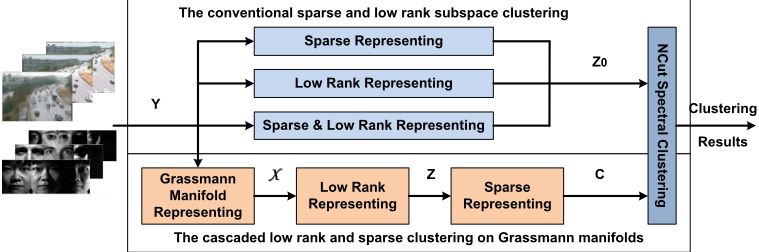
Another observation is that most of the current subspace clustering methods take the data as vectors with Euclidean distance as the metric. However, for many imageset, video data or other multi-dimension data, the simple vectorized data form and its metric are not applicable since it has been proven that many high-dimension data are embedded in lowdimension manifolds with nonlinear metric [Wang et al., 2008]. So it is rational to model such multi-dimension data as manifolds. For this purpose, we adopt the Grassmann manifolds to represent multi-dimension data for clustering, because Grassmann manifolds is a good tool for representing imageset or video data [Turaga et al., 2008] and has a nice property that it can be embedded into the linear space of symmetric matrices. To this end, we further conquer the challenging problem of constructing our CLRSR on the manifold space, which results in a novel data clustering on Grassmann manifolds, called G-CLRSR. We illustrate the main idea of our proposed method in Figure 1 to compare with the conventional sparse and low rank subspace clustering methods.
The contributions of this work are summarized as follows:
- Proposing a novel cascaded low rank and sparse representation model to fully capture the global and local structures underling the observed data;
- Extending the CLRSR model onto Grassmann manifolds which favors the representation of multi-dimension data; and
- Giving a practical solution to the optimization problem on manifold space for the proposed G-CLRSR model.
2 Relevant Concepts
Throughout the paper, all matrices/vectors are written as bold uppercase/lowercase, i.e., X/x. A subscript is used to label the sequence of matrices/vectors, i.e., Xi/xi. Transpose matrix XT and inverse matrix X-1 are also defined. The calligraphic letter X and E represent tensor data and the italic letters (V,N, v) denote scalar values or integers. Other special symbols will be explained when they are used.
2.1 LowRank and Sparse Representation (LRSR)
To explore the hidden global structure, one often enforces the low rank constraint on the self-expression of data. The local neighbor relationship is also critical to subspace clustering; therefore, one joins the neighbor relationship and the global structure to improve the clustering performance [Zhuang et al., 2012; Patel et al., 2015] as,
where Y = [y1, y2, · · · , yN] ∈ Rd×N denotes a set of samples collected from multiple independent subspaces. rank(·) computes the rank of matrix and ℓ0-norm ‖ · ‖0 counts the number of non-zero elements of matrix. The reconstructed error is measured by Euclidean distance.
Different from above LRSR model, our proposed method exploits the sparse representation of the former learned global structure to capture the neighborhood structure. Additionally, to handle multi-dimension data, we further extend it from Euclidean space onto manifold space. Here the Grassmann manifold is adopted.
2.2 GrassmannManifolds
Definition 1 (Grassmann Manifolds) [Absil et al., 2008] The Grassmann manifold, denoted by G(p, n), consists of all the p-dimensional subspaces in n-dimensional Euclidean space Rn (0 ≤ p ≤ n).
To intuitively represent Grassmann manifolds, the popular way is to construct Grassmann manifolds by
From this, we can see that a Grassmannian point actually is an equivalent class (a subset) in which any two thin-tall orthogonal can be converted to each other applying a p×p orthogonal matrix.
Definition 2 (Embedding Distance) [Harandi et al., 2013] Grassmann manifold can be embedded into the symmetric matrices space by
Given two Grassmannian points X1,X2 ∈ G(p, n), the embedding induces the following distance on Grassmann manifolds, defined as,
There exist different types of geometries on Grassmann manifold, please refer to [Absil et al., 2008].
3 Cascaded LowRank and Sparse Representation on Grassmann Manifolds
In this Section, we will elaborate a cascaded version of low rank and sparse representation model for clustering.
3.1 CLRSR on GrassmannManifolds
To explore the global structure, we enforce the low rank constraint on the self-expression coefficients matrix of data. Then to fulfill the local properties, the low rank representation of data is cascaded with the sparse representation. So we have
where λ1, λ2, and λ3 are three major balancing parameters, and the coefficient matrices Z,C ∈ RN×N . This model is named as CLRSR model. As a common precessing, we replace the low rank and sparse items by the nuclear norm and ℓ1-norm as the effective approximations,
To handle multi-dimension data, we consider the generalization of model (6) onto Grassmann manifolds. Given a set of Grassmannian points X = {X1,X2, · · · ,XN} where Xi ∈ G(p, d), the parallelized model is given by
where we use abstract symbols ⊖, ⊎Nj=1 and ⊙ to simulate the "linear" operations to be defined on manifolds, i.e., addition, subtraction and scalar-multiplication. ‖Xi⊖(⊎Nj=1 zij⊙ Xj)‖G measures the error between the Grassmannian point Xi and its "reconstruction" ⊎Nj=1 zij ⊙Xj . According to the property of Grassmann manifolds in (3), it is easy to use the embedding distance to replace the manifold distance as,
where X = {X1XT1 ,X2XT2 , · · · ,XNXTN } is a 3-order tensor and ×3 is the mode-3 tensor-vector multiplication [Kolda and Bader, 2009]. This error measurement not only avoids using Log map operator but also has simple computation with F-norm. Finally, the CLRSR model on Grassmann manifolds can be defined as follows,
where the reconstructed error E is also a 3-order tensor. This model is named as G-CLRSR.
3.2 Optimization
Following the notation used in [Wang et al., 2014], we firstly simplify the tensorial error term E in formula (9) to avoid a complex computation between tensor and matrix,
where E(:, :, i) = XiXTi - ∑Nj=1 zij(XjXTj ) is the ith front slice of E. For convenience, we denote ∆ij = tr[(XTj Xi)(XTi Xj)] and the N × N symmetric matrix ∆ = [∆ij]Ni=1,j=1 . After a sequence of simple mathematical manipulations, we can show that problem (9) is equivalent to
We use Alternating Direction Method [Lin et al., 2011] to solve such a convex problem. For this purpose, we introduce two auxiliary variables J = Z and Q = C to separate variables Z and Q, and reformulate the optimization problem as
which can be solved by minimizing its ALM formula
where A and B are the Lagrange multipliers, and µ is the penalty parameter. The above ALM is appealing on if we can find closed form solutions to the following subproblems (13), (14), (15) and (16).
Updating J. Fixing other variables, we update J by,
A closed-form solution is suggested as the following theorem [Cai et al., 2010],
Lemma 1 Given that UDVT = SVD(Z + Aµ ) as defined above, the solution is given by
where D is the diagonal matrix of singular values. The singular value thresholding operator is defined as Sτ(x) = sign(x) · max(|x| - τ, 0) where τ is a positive number.
Updating Z. To update Z, we solve the following problem by fixing other variables,
This is a quadratic optimization problem with respect to Z. We set its derivation as zero and get the closed solution as,
Updating Q. By fixing other variables, we update Q through,
We know that the problem in (15) has a closed-form solution, given by [Beck and Teboulle, 2009],
Lemma 2 Let matrix M = C+ Bµ and a positive number τ , a closed-form global optimal solution of above problem is
where the singular value thresholding operator is also defined as Sτ = sign(x) · max(|x| - τ, 0).
Updating C. The final self-expression C is updated by solving the following problem,
Similar to update the subproblem Z, we also set the derivation of (16) to zero and get the closed-form solution,
Updating A and B. After we solving the above subproblems on J,Z,Q and C, respectively, we can easily update these two linear Lagrangian multipliers by
Adapting penalty parameter µ. For the penalty parameter µ > 0, we could update it by
where µmax is the pre-defined upper bound of µk .
Once obtaining the coefficient matrix C, any clustering algorithm, i.e., NCut used in this paper, can be performed on affinity matrix W = (|C| + |C|T )/2 to receive final clustering results. We summarize pseudo code in Algorithm 1.
Algorithm 1 The G-CLRSR Optimizing Problem.
Input: Grassmannian points {Xi}Ni=1 , Xi ∈ G(p, d), the balancing penalty parameters λ1, λ2 and λ3. Output: The coefficient matrix C.
- 1: Initialize: J = Z = N = Q = 0, A = B = 0, ρ = 1.1, ϵ = 10-8 , µ0 = 10-6 and µmax = 106 .
- 2: ##Calculating ∆
- 3: for i=1:N do
- 4: for j=1:N do
- 5: ∆ij ← tr[(XjXTj )(XTi Xi)]
- 6: end for
- 7: end for
- 8: ##Optimizing variables
- 9: while not converged do
- 10: Updating variable J,Z,Q,Cvia (13-16), respectively.
- 11: Updating multipliers A and B via (17).
- 12: Updating parameter µ by µ =min(ρµ, µmax).
- 13: Checking the convergence conditions:
- 14: end while
3.3 Complexity and Convergence Analysis
As shown in Algorithm 1, the major time-consuming components lie in steps 5, 10, 11, and 13. (i) The complexity of step 5, the computation of the symmetric matrix ∆, is O(p2d + p3 ) as its main complexity comes from 4 matrices multiplication; (ii) Step 10 takes a SVD operation for updating J, leading to a complexity of O(N 3 ); and (iii) Both steps 11 and 13 involve matrix multiplication and inversion operations, thus the complexity is O(N 3 ). Overall, the total complexity is O(N 2 (p2d + p3 ) +N 3 ) for each iteration. Under the condition p ≪ d, the total complexity is basically O(N 2 p2d + kN 3 ) where k denotes the number of iterations.
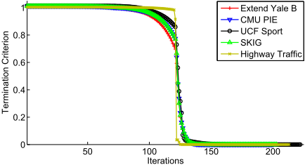
To experimentally show the convergence behavior of the proposed method, we provide an intuitive curve illustration of the convergence with respect to the iteration number on all datasets, shown in Figure 2. Our proposed algorithm converges in about 230 steps, which reflects that our optimization method has a good convergence property.
4 Experiments
4.1 Datasets
Extended Yale B dataset is collected from 38 subjects and each subject has 64 front face images. We randomly choose 8 images from the same subject to construct an imageset.
CMUPIE 1 dataset contains totally 1632 front face images evenly from 68 subjects. Every 4 images from the same subject are chosen to construct an imageset.
UCF sport dataset 2 includes a total of 150 video clips with 13 actions, which has a wide range of scenes and viewpoints. Each clip has 22 to 144 frames.
SKIG gesture dataset 3 contains 1080 RGB-D video clips with 10 gesture types of 6 subjects. All the gestures are performed under different backgrounds and illumination. Each sequence contains 63 to 605 frames.
Highway traffic dataset 4 contains 253 video clips labeled with three levels. Each clip has 42 to 52 frames.
Each video clip is regarded as an imageset to construct a point on Grassmann manifolds.
4.2 Comparison Algorithms and Settings
For the comparison algorithms, we have the following (i) vector-form input methods, LRR [Liu et al., 2013], SSC [Vidal, 2011], LS3C [Patel et al., 2013] and CLRSR, (ii) Grassmann-form input methods, SCGSM [Turaga et al., 2011], SLRR [Yin et al., 2015], FGLRR [Wang et al., 2014], LapFGLRR [Wang et al., 2018] and a baseline G-LRSR.
To execute LRR, SSC, LS3C and LRSR on imageset and video data, we have to vectorize each imageset as inputs for them. However, in most experiments, we cannot simply take these long vectors into the algorithms due to the high dimension for a larger imageset. So, we reduce the dimension of these vectors to a low one which equals to the dimension of PCA components retaining 95% of its variance energy.
SLRR extends LRR onto Stiefel manifolds which has the same form with Grassmann manifolds. SCGSM and FGLRR can be considered as the Grassmann manifolds version of Kmeans and LRR models. In LapFGLRR, a local constraint among data, Laplacian regularization, is introduced into the FGLRR model. In G-LRSR, the LRSR model is embedded into Grassmann manifolds as a important baseline.
For a fair comparison, we execute the code of compared methods provided by authors. The parameters λ1, λ2 and λ3 in CLRSR and G-CLRSR, one parameter λ1 in LRR, SSC, FGLRR and SLRR, two parameters λ1 and λ2 in LapFGLRR, G-LRSR and LS3C, need to be tuned, respectively. We tune their values within the set of {0.1, 0.2, · · · , 1, 2, · · · 10}, and we report the best value in each experiment.
To make a comprehensive evaluation, we employ five clustering validation measurements, including ACC (accuracy), NMI (normalized mutual information), RI (rand index), Purity and FM (F-measure). For all the metrics, higher values indicate better performance.
1 http://www.cs.cmu.edu/afs/cs/project/PIE/MultiPie/Multi-
Pie/Home.html
2 http://crcv.ucf.edu/data/
3 http://lshao.staff.shef.ac.uk/data/SheffieldKinectGesture.htm
4 http://www.svcl.ucsd.edu/projects/traffic/
4.3 Data Representation
An imageset F = {f1, · · · , fP}; fi ∈ Rd , with fi being the feature descriptors of i-th frame. In this paper, we just use the image intensity as the raw feature. The Grassmannian point can be represented by an orthogonal basis. Similar to the work in [Wang et al., 2014], the feature matrix F ∈ Rd×P is decomposed by SVD as F = UΣVT ; then we pick up the first p (p ≤ P) singular-vectors of U to represent a point X = [u1, u2, ..., up] on Grassmann manifolds G(p, d).
4.4 Experimental Results
Image Set Data Clustering
Although facial recognition and clustering has been a mature application in computer vision, it often gets unfavorable experimental results since the varieties of facial expressions, poses or light conditions. Imageset data collect complementary information from multiple views of each object, which can naturally overcome the environment affection. Here, we regard each imageset as one point on Grassmann manifolds.
Table 1 reports all clustering results in terms of different validation criteria on two facial imageset datasets. From an overall perspective, manifold representation based methods obtain better performance than vector-form input clustering methods (i.e., LRR, SSC and LS3C), which demonstrates that manifold representation is a good tool for imageset data. Compared with SLRR, SCGSM and FGLRR, our proposed method simultaneously considers meaningful global and neighbor structures, which makes our proposed method more robust in clustering tasks. As for the important baselines, i.e., LapFGLRR and G-LRSR, they both involve global and local constraints on only one layer of representation, while our proposed approach can extract meaningful representation layer by layer. Through keeping the local neighbor relation on the base of global structure information, our proposed method receives the best experimental results.
Video Data Clustering
Action recognition is another open and hot issue in computer vision literature. Most action data are in the form of video clips, which is a set of sequential frame images and suitable to our manifold representation methods. So we select a human action and a gesture video datasets.
Table 2 lists the results of different clustering methods on video datasets. These datasets are much more challenging than the previous two fical imageset datasets, as the environment is more complex and varies dramatically. Obviously, for video datasets, manifold representation based methods reflect more impressive superior to vector-input based methods, which is further to verify the advantage of manifolds representation. What is more, LapFGLRR, G-LRSR and our proposed methods report the superior results in all five metrics, which also verify that fusing global and local information are important for video data on clustering tasks. It should be noted that the performance of most compared methods are not robust to all datasets. For example, LapFGLRR achieves the best performance on SKIG in terms of RI . However, the performance on the other datasets are not such promising.
In addition, we wish to evaluate our proposed method in a real and practical application; therefore, a natural scenario dataset, Highway Traffic videos, is chosen as test data. Table 3 shows the clustering results of all the algorithms, our proposed method still get satisfied performance, i.e., almost 4 percent rasing performance in ACC. For the general application of G-CLRSR, we can use it to learn the threshold of different level or part the period for the traffic jam on specific roads based on the historical traffic data.
| Method | Extended YaleB | CMUPIE | ||||||||
|---|---|---|---|---|---|---|---|---|---|---|
| ACC | NMI | RI | Purity | FM | ACC | NMI | RI | Purity | FM | |
| LRR | 47.47 | 67.80 | 96.23 | 49.49 | 6.74 | 40.59 | 73.12 | 97.69 | 43.82 | 2.84 |
| SSC | 39.06 | 62.25 | 96.22 | 42.42 | 3.14 | 51.18 | 77.97 | 98.26 | 52.06 | 3.47 |
| LS3C | 22.56 | 48.14 | 95.25 | 22.90 | 3.15 | 26.18 | 62.89 | 97.46 | 27.35 | 1.50 |
| CLRSR | 38.05 | 62.23 | 95.97 | 40.74 | 6.11 | 27.06 | 63.44 | 97.45 | 28.82 | 3.62 |
| SLRR | 55.56 | 73.14 | 97.04 | 57.58 | 6.71 | 24.21 | 61.63 | 97.36 | 25.88 | 1.53 |
| SCGSM | 39.06 | 62.83 | 95.51 | 41.75 | - | 14.41 | 42.31 | 90.89 | 15.59 | - |
| FGLRR | 80.81 | 88.93 | 98.71 | 81.48 | 19.75 | 61.47 | 81.02 | 98.53 | 63.53 | 7.09 |
| LapFGLRR | 77.10 | 87.31 | 98.43 | 78.11 | 18.18 | 57.35 | 79.36 | 98.30 | 59.71 | 6.45 |
| G-LRSR | 78.45 | 88.62 | 98.43 | 80.13 | 17.95 | 45.29 | 73.74 | 97.86 | 48.24 | 3.96 |
| G-CLRSR | 81.82 | 90.20 | 98.78 | 82.83 | 22.22 | 62.94 | 81.74 | 98.56 | 64.71 | 7.35 |
| Method | UCF Sport | SKIG | ||||||||
|---|---|---|---|---|---|---|---|---|---|---|
| ACC | NMI | RI | Purity | FM | ACC | NMI | RI | Purity | FM | |
| LRR | 42.67 | 47.56 | 81.49 | 46.00 | 16.67 | 25.00 | 33.16 | 72.23 | 29.44 | 19.25 |
| SSC | 58.00 | 63.79 | 91.13 | 64.00 | 25.29 | 38.89 | 47.62 | 85.95 | 42.41 | 1.78 |
| LS3C | 55.33 | 63.25 | 90.70 | 62.67 | 24.18 | 28.33 | 33.72 | 81.60 | 30.00 | 19.96 |
| CLRSR | 50.00 | 56.14 | 88.13 | 55.33 | 25.74 | 20.93 | 13.17 | 82.44 | 22.22 | 18.56 |
| SLRR | 74.00 | 76.29 | 94.41 | 75.33 | 40.00 | 41.30 | 44.96 | 86.21 | 42.59 | 14.32 |
| SCGSM | 66.67 | 76.17 | 92.59 | 71.33 | 32.43 | 29.26 | 42.44 | 81.35 | 34.81 | 18.03 |
| FGLRR | 76.00 | 86.01 | 95.09 | 82.00 | 43.75 | 50.19 | 54.50 | 88.33 | 52.04 | 15.43 |
| LapFGLRR | 79.33 | 86.47 | 95.52 | 82.00 | 47.46 | 50.74 | 54.11 | 88.50 | 55.56 | 20.07 |
| G-LRSR | 76.00 | 82.47 | 95.03 | 79.33 | 41.94 | 46.11 | 53.57 | 86.98 | 51.30 | 15.87 |
| G-CLRSR | 81.33 | 86.69 | 96.11 | 84.00 | 50.00 | 50.93 | 56.77 | 85.77 | 56.11 | 21.76 |
| Method | ACC | NMI | RI | Purity | FM |
|---|---|---|---|---|---|
| LRR | 67.59 | 35.75 | 68.50 | 69.96 | 50.60 |
| SSC | 60.47 | 57.10 | 73.36 | 81.42 | 46.24 |
| LS3C | 70.36 | 26.34 | 66.71 | 71.15 | 46.45 |
| CLRSR | 66.80 | 12.73 | 60.06 | 67.98 | 36.36 |
| SLRR | 64.82 | 34.18 | 62.63 | 75.49 | 43.43 |
| SCGSM | 79.84 | 52.59 | 82.72 | 80.63 | 61.65 |
| FGLRR | 80.24 | 58.51 | 87.39 | 81.82 | 47.95 |
| LapFGLRR | 81.42 | 60.99 | 86.94 | 82.21 | 64.66 |
| G-LRSR | 73.12 | 61.90 | 78.08 | 81.82 | 48.89 |
| G-CLRSR | 85.38 | 60.01 | 87.39 | 85.38 | 66.67 |
5 Conclusion
In this paper, we proposed a novel cascaded low rank and sparse representation clustering method and extended it onto Grassmann manifolds to handle multi-dimension or imageset data. Compared with existing works which integrate low rank and sparse constraints on the same data representation simultaneously, the proposed methods execute a sparse constraint on the low-rank representation matrix in a cascaded manner which contributes to obtaining an improved affinity matrix. In addition, an efficient alternative based algorithm is proposed to solve for the optimal solution. Intensive experiments were conducted on imagesets and video datasets to demonstrate the superior performance of our methods.
Acknowledgements
The research project is supported by the Australian Research Council (ARC) through the grant DP140102270 and also partially supported by National Natural Science Foundation of China under Grant No. 61390510, 61672071, 61632006, 61772048, Beijing Natural Science Foundation No. 4172003, 4162010, 4152009, 4184082, Beijing Municipal Science and Technology Project No. Z171100000517003, Z171100000517004, Z171100004417023, Z161100001116072.
@inproceedings{ijcai2018p382,
  title     = {Cascaded Low Rank and Sparse Representation on Grassmann Manifolds},
  author    = {Wang, Boyue and Hu, Yongli and Gao, Junbin and Sun, Yanfeng and Yin, Baocai},
  booktitle = {Proceedings of the Twenty-Seventh International Joint Conference on
               Artificial Intelligence, {IJCAI-18}},
  publisher = {International Joint Conferences on Artificial Intelligence Organization},
  editor    = {Jérôme Lang},
  pages     = {2755--2761},
  year      = {2018},
  month     = {7},
  note      = {Main track},
  doi       = {10.24963/ijcai.2018/382},
  url       = {https://doi.org/10.24963/ijcai.2018/382},
}
TY - CPAPER TI - Cascaded Low Rank and Sparse Representation on Grassmann Manifolds AU - Wang, Boyue AU - Hu, Yongli AU - Gao, Junbin AU - Sun, Yanfeng AU - Yin, Baocai T2 - Proceedings of the Twenty-Seventh International Joint Conference on Artificial Intelligence, IJCAI-18 PB - International Joint Conferences on Artificial Intelligence Organization PY - 2018 SP - 2755 EP - 2761 DO - 10.24963/ijcai.2018/382 UR - https://doi.org/10.24963/ijcai.2018/382 ER -Copied
Machine-readable versions of this paper, for tools and AI agents:





