When Rigging a Tournament, Let Greediness Blind You

1 Introduction

A knockout tournament is a standard format of competition, consisting of several rounds. In each round, all players that have not yet been eliminated are paired up into matches. Losers are eliminated, and winners are raised to the next round, until only a single winner exists. For an illustrative example, consider Wimbledon Men's tennis tournament (having 128 players). In fact, knockout tournament is the most widely-used format of competition in sports [Horen and Riezman, 1985; Connolly and Rendleman, 2011; Groh et al., 2012]. Apart from sports and popular culture, knockout tournaments are also prevalent in elimination-based election and decision making schemes. Specifically, they received notable attention from the viewpoints of artificial intelligence [Vu et al., 2009; Williams, 2010; Stanton and Williams, 2011c; 2011b; 2011a; Aziz et al., 2014; Michael et al., 2016; Kim and Williams, 2015; Ramanujan and Szeider, 2017] as well as economics and operation research [Rosen, 1986; Tullock, 1980; Laslier, 1997].

Having a favorite player v⋆ in mind, is there a way to conduct the competition so that v⋆ wins? To formulate this question formally, note that the execution of a knockout tournament with a set N of N players is governed by a complete (unordered) binary tree T with n leaves and a mapping ϕ : N → leaves(T), called a seeding. In the first round, every two players mapped to leaves with the same parent compete against each other, and the winner is mapped to the common parent. The leaves are then deleted from the tree, and the next round is conducted similarly. The execution stops when the tree contains a single vertex, mapped to a player who is declared the winner. The question of making v⋆ a winner is sensible when we have predictive information about outcomes of matches. Specifically, we assume we have a tournament D = (V, A) (not to be confused with the competition itself that is also termed a tournament), which is a digraph where either (u, v) ∈ A or (v, u) ∈ A for all u, v ∈ V . This encodes predictive information as follows : V = N, and for every u, v ∈ N, we predict that in a match between u and v, u would beat v if and only if (u, v) ∈ A.

Now, our question is formalized as follows.

TOURNAMENT FIXING PROBLEM (TFP)

Input: A tournament D = (V, A), and a vertex v⋆ ∈ V .

Parameter: The feedback arc set number k⋆ of D.

Question: Is there a seeding of the n = |V | players such

that v⋆ wins the resulting knockout tournament?

The problem of rigging a knockout tournament was introduced by Vu et al. [Vu et al., 2009]. This work led to a flurry of research of structural properties of D that guarantee that v⋆ wins [Michael et al., 2016; Kim and Williams, 2015; Stanton and Williams, 2011c; 2011b; 2011a; Aziz et al., 2014; Michael et al., 2016; Williams, 2010]. Additional information can be found in surveys such as [Williams, 2016]. The question of whether TFP is NP-hard was posed in several works, including [Vu et al., 2009; Williams, 2010; Russell and Beek, 2011; Stanton and Williams, 2011b; 2011c; 2011a;

Lang et al., 2012]. It was finally resolved in the affirmative by Aziz et al. [Aziz et al., 2014], showing that it can be solved in time O(2.83n ). Later, Kim and Williams [Kim and Williams, 2015] gave an O(2n ) time and space algorithm. Even for a small number of players, such a running time is prohibitive. Moreover, approximation of TFP does not make sense.

In light of the discussion above, a most natural framework to study TFP is parameterized complexity. Specifically, Aziz et al. [Aziz et al., 2014] considered the feedback arc set number of D as the parameter k⋆ . This parameter has a natural interpretation. It is likely that in real world scenarios, there is an approximate ranking of players' strengths (e.g., Wimbledon), so that a player of a certain rank is expected to beat players of a lower rank. The number of matches where we guess (before the competition begins) that a player of a certain rank will beat a player of higher rank, which upper bounds k⋆ , is significantly smaller than n.

In the last decade, parameterized complexity has transformed into a rich and vibrant field, being one of the most intensively studied areas in theoretical computer science (see fpt.wikidot.com/fpt-papers-in-conferences). With some delay, using methods in parameterized complexity to resolve problems in social choice theory is also becoming common. In particular, this line of attack has been proven particularly successful in voting theory (see, e.g., [Bulteau et al., 2015; Bredereck et al., 2016; Dey et al., 2017; Bredereck et al., 2014b; Dey et al., 2016; Chen et al., 2017; Bredereck et al., 2014c; 2014c]); for more information on the current state-ofthe-art, we refer to excellent surveys such as [Bredereck et al., 2014a; Betzler et al., 2012; Faliszewski and Niedermeier, 2016; Fischer et al., 2016].

Aziz et al. [Aziz et al., 2014] showed that TFP is XP, which means solvability in time nf(k⋆ ) for some function f of k⋆ . They gave a clever dynamic programming algorithm that runs in time nO(k⋆ ) . Assuming that k⋆ is not fixed (i.e., independent of n), such a running time is again prohibitive. The question of whether TFP is fixed-parameter tractable with respect to k⋆ , that is, solvable in time f(k⋆ )nO(1) for some function f, was later resolved by Ramanujan and Szeider [Ramanujan and Szeider, 2017]. They showed that TFP is solvable in time 2O(k⋆2 log k⋆ )nO(1) . This means that whenever k⋆2 log k⋆ = O(log n), TFP is solvable in polynomial time.

1.1 Our Contribution

The main component of the algorithm by Ramanujan and Szeider [Ramanujan and Szeider, 2017] is the translation of TFP into an algebraic system of equations, solved in a black box fashion by an ILP solver. In particular, the algorithm (and not just the proof of correctness) by Ramanujan and Szeider [Ramanujan and Szeider, 2017] is thus both complicated and not self-contained. We present a fresh greedy solution whose correctness relies on new insights into TFP itself. The advantages of our algorithm are as follows.

First, our algorithm is purely combinatorial (unlike the algebraic algorithm of [Ramanujan and Szeider, 2017]). While the analysis of our algorithm is intricate, the algorithm itself is simple and easily implementable. Essentially, after we "guess" a template tree (similarly to [Ramanujan and Szeider,

2017]), our algorithm merely iterates over the paths and subtrees that are not already determined by the guess, and fills them up in a greedy manner. We find it both surprising and pleasing that such a strategy just works. From our proof of correctness, the reasons for the validity of this strategy are revealed, but at first glance, we do not find them apparent.

Second, our solution is completely self-contained. We do not invoke any black-box ([Ramanujan and Szeider, 2017] invokes a big hammer, i.e., an ILP solver).

Third, our algorithm is substantially faster than that of [Ramanujan and Szeider, 2017]. Specifically, our running time bound is 2O(k⋆ log k⋆ )nO(1) rather than 2O(k⋆2 log k⋆ )nO(1) . The difference is clear already for values as small as k⋆ = 8, where 2k⋆ log2 k⋆ = 224 while 2k⋆2 log2 k⋆ = 2192 . Even for k⋆ = 4, 2k2 log2 k = 232 >> 224 . Thus, it is very plausible that our improvement constitutes the difference between being practically infeasible and feasible for social choice applications, where n typically ranges between a few tens to a few hundreds, if k⋆ is presumed to be, say, 5% of n. In a different view, our result also proves that whenever k log k = O(logn), TFP is solvable in polynomial time.

Proofs omitted entirely are denoted by ⋆.

2 Preliminaries

Let [n] = {1, . . . , n}. Given a tournament D, let V (D) and A(D) denote its vertex set and arc set, respectively. For a pair of vertices u, v, by (u, v) we denote an arc from u to v, and say that u is an in-neighbor of v and v is an out-neighbor of u. A uv-path is a path from u to v. Given X ⊆ V (D), by D[X] we denote the subtournament of D induced by X and N(X) is the set of neighbors of the vertices in X outside X. For a rooted tree T and a vertex v ∈ V (T), by Tv we denote the subtree of T rooted at v. An arborescence is a rooted directed tree such that all arcs are directed away from the root.

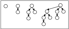
We now discuss the notion of a binomial arborescence and its relevance to our work (see Fig. 1.).

Definition 1. An unlabeled binomial arborescence (usba) T rooted at v ∈ V (T ) is defined recursively as follows:

• A single node v is a binomial arborescence rooted at v.
• Given two vertex disjoint binomial arborescences of equal size, Tv rooted at v and Tu rooted at u, adding an arc from v to u results in a binomial arborescence T rooted at v.

Let D be a directed graph. If T is a subgraph of D with V (T) = V (D), then T is a labeled spanning binomial arborescence (sba) of D.

Given an integer n = 2j , there exists a unique usba, denoted by Bn, on n vertices. For our purpose, we fix a labelling of the vertices of Bn from [n], that is, a function

γ : V (Bn) → [n]. Whenever we refer to an usba on n vertices, we always mean Bn, where the vertices are labeled by γ. Our interest in sba is due to the following connection between sba and finding a seeding of the vertices in D that results in a specific vertex being the winner.

Proposition 1 ([Williams, 2010]). Let D be a tournament with v⋆ ∈ V (D). There is a seeding of the vertices in D such that the resulting knockout tournament is won by v⋆ if and only if D has a sba rooted at v⋆ .

Proposition 1 reduces TFP to the problem of finding a sba rooted at v⋆ . Throughout, we take this view of the sba problem. In this context, the following lemma will come in handy.

Lemma 1 (⋆). Let D be a tournament, X ⊆ V (D) such that D[X] is acyclic, and T be arborescence on |X| vertices. Then, D[X] contains (as a subgraph) an arborescence isomorphic to T that can be computed in polynomial time.

Next, we give some simple properties of sba.

Observation 1 ([Ramanujan and Szeider, 2017]). Let B be an sba on n vertices. Then, the height of B (the maximum length of a path from root to leaf) is logn. Moreover, for any vertex v in B, the number of children of v is at most log n, and the size of the subtree of B rooted at v is one of the following numbers: 20 , 21 , · · · , 2logn .

3 Greedy Algorithm for TFP

As stated earlier, due to Proposition 1, we study the following equivalent question: Does there exist an sba rooted at v⋆ in D? We start by computing a minimum sized feedback arc set, F , of D. It is well known that a tournament has a directed cycle if and only if it has a directed triangle. Furthermore, a subset F of A(D) is a minimal feedback arc set if and only if the tournament Drev obtained after reversing the arcs in F is acyclic. Using these two facts, one can design a trivial branching algorithm for finding F running in time 3k⋆ nO(1) . That is, while there exists a triangle in the given tournament, find one and recursively try to find a smaller sized solution by reversing an arc of the triangle. See [Cygan et al., 2015] for further details. In fact one can find a minimum sized feedback arc set, F, of D in time 2O(√k⋆ )nO(1) [Feige, 2009; Karpinski and Schudy, 2010]. From now onwards, we assume that we have a feedback arc set F at hand.

Let σ be the topological ordering of D after reversing the arcs in the feedback arc set F. Throughout the paper, we always work with the topological ordering σ. If a vertex v precedes u in σ, then we write v ≺σ u. Given V ′ ⊆ V (D), the highest vertex in V ′ is the vertex that precedes all other vertices of V ′ in the ordering σ. Furthermore, for any arc (u, v), we say that u beats v (equivalently, v is beaten by u). We now give a few basic definitions central to our algorithm.

Definition 2. (LCA closure) For a rooted tree T and a vertex subset M ⊆ V (T), the least common ancestor-closure (LCA-closure) LCA(M) is obtained by the following process. Initially, set M ′ = M. Then, as long as there are vertices x and y in M ′ whose least common ancestor w in T is not in M ′ , add w to M ′ . When the process terminates, output M ′ as the LCA-closure of M.

The following folklore lemma (see, e.g., [Cygan et al., 2015]) summarizes two basic properties of LCA closures.

Lemma 2. Let T be a rooted tree, M ⊆ V (T) and M ′ = LCA(M). Then |M ′ | ≤ 2|M| and for every connected component C of T \M ′ , |N(C)| ≤ 2.

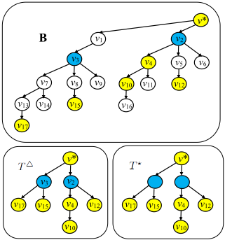
Our algorithm will "guess" some information about a solution (if one exists), and then greedily complete the parts unknown. To discuss these guesses (Phase 1), we require the following definition (see Fig. 2).

Definition 3. (Topology and Template) Let B be an sba rooted at v⋆ and let X ⊆ V (B). We construct a tree T △ from B as follows. First delete all vertices that do not lie on any v⋆u-path in B for any u ∈ LCA(X). Now, as long as there is a vertex u ∈ V (B) \ LCA(X) with exactly one in-neighbor u- and exactly one out-neighbor u+, delete the vertex u and add the arc (u-, u+). Then T △ is a tree obtained at the end of this process, it is called the topology of X in B. The template tree of X in B is a tree obtained from T △ by deleting the labels of all vertices in LCA(X) \ X. A tree T ⋆ is a template of X if it is a template of X in at least one sba B rooted at v⋆ .

Before going further, we recall some notation.

Let F denote the feedback arc set and VF denote the set of vertices that are adjacent to arcs in F. We denote k = |VF |. Observe that k ≤ 2k⋆ . Furthermore, σ denote the topological ordering of D after reversing the arcs in F .

For the phases where we complete missing information, the following definition will be crucial.

Definition 4. (Fas-vertex, Fas-parent and Fas-child) Let T ⋆ be a template of VF ∪ {v⋆ }. Vertices in VF ∪ {v⋆ } are called fas-vertex. Let v ∈ V (D). The fas-parent of v is the last fas-vertex w not equal to v on the v⋆ v-path in T ⋆ . An fas-child of v is an fas-vertex w, that is the first fas-vertex not equal to v on the vw path in T ⋆ . The set of fas-children of v in T ⋆ is denoted by faschild(v).

As a first step, our algorithm would need to enumerate all templates of VF ∪ {v⋆ }. Due to Lemma 2, a template of VF ∪ {v⋆ } in any sba is a rooted tree T on at most 2k + 1 vertices with some of its vertices labeled with the vertices in VF ∪ {v⋆ } and the others unlabeled, beings placeholder for LCA vertices. We can therefore enumerate a superset of templates by enumerating every rooted tree on at most 2k +1 vertices with a surjective mapping of some of its vertices to vertices in VF ∪ {v⋆ } such that the root is mapped to v⋆ , and all the leaves are mapped as well (to vertices in VF ∪ {v⋆ }):

Observation 2. A superset of the set of templates of VF ∪ {v⋆ } of size kO(k) can be enumerated in time kO(k) .

Intuition. Our algorithm proceeds in four steps. First, we guess a partial structure of the sba. Second, we verify that the guesses made in the previous step are "realizable". These two steps are straightforward, and are also present in a similar form in [Ramanujan and Szeider, 2017]. Then, we turn to the heart of our algorithm. Here, we design a "greedy" procedure to complete the partial sba in two steps. The first fills up paths corresponding to edges of the template at hand. Roughly speaking, here we always select a yet "unhandled" fas-vertex v that is highest in V (D) with respect to σ. Then, we greedily fill the path between v and its fas-parent using the highest "available" vertices that are "between" v and its fasparent (i.e., beat v and beaten by the parent). This is a slight simplification since when we look at the path between v and its fas-parent, a part of it (closer to the parent) is already filled. However, by considering lca vertices this technicality is easily handled. The second phase fills-up the subtrees hanging from the paths we have just filled. Roughly speaking, while we still have an unfilled subtree, we pick one that hangs from a vertex v that is highest. We greedily fill the subtree with "available" vertices that are the highest ones beaten by v. If the greedy procedure ever gets stuck, we move to the next partial sba. While the procedure itself is very simple, correctness is surprising, and indeed the proof is quite intricate.

3.1 Phase I: Guessing

We first intuitively explain what we intend to achieve by guessing. Suppose I = (D, v⋆ , k) is a YES-instance of TFP. Then, there exists an sba B rooted at v⋆ . We first guess the template T ⋆ of VF ∪ {v⋆ } in B. Given T ⋆ , for each arc (u, v), we guess a length, denoted by len(u, v), that is the number of internal vertices on the unique uv-path in B. Then, for each vertex v ∈ VF , we guess the size of the subtree rooted at v in B, denoted by siz(v). Due to Observation 1, len(u, v) ∈ {0, · · · , logn} and siz(v) ∈ {20 , 21 , · · · , 2logn }. Formally, in this phase we guess the following.

1. Using Proposition 2, we iterate over all templates of VF ∪ {v⋆ }. Let T ⋆ denote one such template.
2. For each arc (u, v) in A(T ⋆ ), guess an integer in {0, · · · , logn}. Formally, we enumerate over all possible "length functions" len : A(T ⋆ ) → {0, · · · , log n}.
3. Next, we guess the "size function". That is, we enumerate all possible functions siz : VF → {20 , · · · , 2log n }.

Definition 5. An sba B complies with (T ⋆ , len, siz) if (i) the template of VF ∪ {v⋆ } in B is T ⋆ , (ii) for each arc

(u, v) ∈ A(T △) where T △ is the topology of VF ∪ {v⋆ } in B,the number of internal vertices on the unique uv-path in B is len(u, v), and (iii) for every v ∈ VF ∪ {v⋆ }, the size of the subtree rooted at v in B is siz(v).

As we do exhaustive guessing, the following is immediate. Lemma 3. If (D, v⋆ , k) is a YES-instance of TFP, there exists an sba B that complies with some tuple (T ⋆ , len, siz) we enumerate.

3.2 Phase II: Verification of Guesses

In this section, we give an algorithm to check whether a guessed tuple (T ⋆ , len, siz) is "realizable". We first define the verification operations we perform on a tuple (T ⋆ , len, siz).

Definition 6 (Realizability). A tuple (T ⋆ , len, siz) is realizable if there is a usba B on n vertices with an injective function φ : V (T ⋆ ) → [n] satisfying the properties below. 1

1. v⋆ is the root of B, that is, φ maps v⋆ to the root of B.
2. T ⋆ is the template of VF ∪ {v⋆ } in B.
3. For each (u, v) ∈ A(T ⋆ ), len(uv) is equal to the number of internal vertices on the uv-path in B.
4. For each v ∈ VF ∪{v⋆ }, siz(v) is equal to the size of the subtree rooted at v in B.

Lemma 4 (⋆). There is a polynomial-time algorithm that checks whether a given tuple (T ⋆ , len, siz) is realizable by at least one pair (B, φ), and if the answer is positive, outputs such a pair.

3.3 Phase III: Greedy Choice for Path Resolution

Given a tuple (T ⋆ , len, siz), we use a greedy strategy to construct an sba B such that (T ⋆ , len, siz) is realizable by B (if one exists). As a preprocessing step, for every arc (u, v) ∈ A(T ⋆ ) with u, v ∈ VF ∪ {v⋆ } and len(u, v) = 0, we check that indeed (u, v) ∈ A(D). If this is not the case, then we conclude that there is no sba that complies with (T ⋆ , len, siz).

Now, recall that our greedy algorithm proceeds in two steps. First, we substitute each arc (v, u) in T ⋆ by a path, which brings us closer to uncovering some sba B. In this section, we only consider the procedure to fill-up these paths. Specifically, given the template T ⋆ , we will construct a tree T that is a template of a superset of VF ∪ {v⋆ }. In particular, it will be a template of V (T) itself.

The tree we construct in the process is referred to as T. Initially, T = T ⋆ . For an arc (u, v) ∈ A(T ⋆ ), we call (u, v) resolved if it has been replaced by a path in T that has len(uv) internal vertices. An fas-vertex v is called resolved if either it is the root (v⋆ ) or all the arcs on the path from its fas-parent, w, to v are resolved. We call a vertex v ∈ V (D) \ VF available if v ∈ V \ V (T). That is, as vertices are added to T to fill the paths corresponding to arcs in V (T ⋆ ), they become unavailable. A vertex is the highest available vertex in X ⊆ V (D) if it precedes all other available vertices in X according to σ.

With this notation, we repeat procedure PathGreedy until all arcs are resolved. Note that in one step (that is, one execution of the procedure), several arcs of A(T ⋆ ) can be resolved.

1 Here, we abuse notation: if a vertex v in T ⋆ is mapped (by φ) to some vertex i ∈ [n] in B, we refer to i as v.

PathGreedy:

1. Let v be the highest unresolved fas-vertex in T ⋆ and w be its fas-parent.
2. Consider the wv-path (Pwv) in T (not in T ⋆ ). Note that in each step we always resolve all the arcs of a path simultaneously. So the set of unresolved arcs on the path Pwv form a subpath of Pwv that ends at v. Let x be the first vertex on the path Pwv such that the no arc on the unique xv-path (Pxv) in T is resolved.
3. Let H be the set of available vertices between x and v in the ordering σ. If |H| ≥ η = ∑(a,b)∈A(Pxv) (len(ab) + 1) - 1, then let H′ denote the subset of H consisting of highest η vertices in it. Then, we replace the path Pxv by the path P ′xv , which consists of vertices in H′ : in the path P ′xv , the vertices in H′ are ordered from highest to lowest rank.
4. If |H| < η, return that there is no sba that complies with (T ⋆ , len, siz).

Let T i denote the tree T that we had at hand immediately after we resolved the ith vertex. The root is automatically resolved, and hence T 1 = T ⋆ . Note that T k+1 = T. We say that PathGreedy fails in step i, if it concludes in ith step (step in which it resolves the ith vertex) that no sba complies with (T ⋆ , len, siz), and else we say that it succeeds in ith step. We say that PathGreedy fails if it concludes that no sba complies with (T ⋆ , len, siz) in some step, and else we say that it succeeds. To argue about the correctness of our greedy choices, we need to extend Definition 5.

Definition 7. An sba B complies with T i if it complies with (T ⋆ , len, siz) and the template of V (T i ) ∩ V (D) in B is T i .

The main components of proof are Lemmata 5 and 6.

Lemma 5 (⋆). Suppose that PathGreedy succeeds up to step i for some i ∈ [k]. Let B be an sba that complies with T i . Then, PathGreedy succeeds at step i + 1.

For the sake of clarity, before we present Lemma 6, we define a procedure used only for analysis. Suppose that PathGreedy succeeds up to step i + 1. Here, suppose we have some sba B that complies with T i for some i ∈ [k]. As PathGreedy succeeds at step i+1, T i+1 is well defined. Let v, x,H ′ , Pxv and P ′xv be as defined in step i + 1 of PathGreedy. Now, supposing that B does not comply with T i+1 , there exists a vertex p on the unique xv-path in B that does not belong to H′ , and a vertex q ∈ H′ that does not belong to the unique xv-path in B. Since the length of these paths are same we have that the only way the last assertion can be violated if both these paths use the same set of vertices but in different order. However, this is not possible since D[H′ ] is a transitive tournament and thus there is a unique directed path spanning all the vertices in H′ . Having these (hypothetical) elements at hand, we consider procedure PathAnalysis.

Lemma 6 (⋆). Assume PathGreedy succeeds up to step i + 1, and let B, v, x,H ′ , Pxv, P ′xv , p, q be as above. If B does not comply with T i+1 , then if these elements are the input to PathAnalysis, it returns B⋆ that is an sba with the following properties: (i) it complies with T i ; (ii) the number of vertices

PathAnalysis:

1. Let Q = x → u1 → · · · → uη → v be the unique xv-path in B. (This is well defined as B complies with T i .)
2. For all i ∈ [η], let u′i be the ith highest vertex in ({u1, . . . , uη} \ {p}) ∪ {q} according to σ.
3. For all i ∈ [η], put u′i in place of ui in B, and put p in (the original) place of q in B. Denote the result by B′ .
4. As long as p has a child r′ in B′ such that (r′ , p) ∈ A(D), let r be the highest such child according to σ, and swap p and r. Denote the result by B⋆ .
5. Return B⋆ .

on the unique xv-path in B⋆ from H′ is larger by 1 than the number of vertices on the unique xv-path in B from H′ .

From Lemma 6, we derive the following consequence.

Corollary 1 (⋆). Suppose that PathGreedy succeeds up to step i + 1. If there is an sba B that complies with T i , then there is an sba B⋆ that complies with T i+1 .

Having the lemma above at hand, our proof is done by induction. For the sake of clarity, let us extract the claim.

Lemma 7 (⋆). For all i ∈ [k + 1], if there is an sba B complying with (T ⋆ , len, siz), then (i) PathGreedy succeeds up until step i, and (ii) there is an sba that complies with T i .

As a corollary to Lemma 7, we obtain the following.

Corollary 2. If there is an sba B complying with (T ⋆ , len, siz), then (i) PathGreedy succeeds, and (ii) there exists an sba that complies with T .

Let us also explicitly state an observation that directly follows from our construction. (Here, correctness also relies on our preprocessing step.)

Observation 3. If PathGreedy succeeds, then T is a subtree of D, and in particular A(T ) ⊆ A(D).

3.4 Phase IV: Greedy Choices for Subtree Resolution

Because we managed to reach this phase, we have at hand (i) a pair (B, φ) that realizes (T ⋆ , len, siz) (from Phase II), and (ii) the tree T outputted by GreedyPaths (from Phase III). Before we proceed to our greedy choices, let us first update (B, φ) to (B⋆ , φ⋆ ) as follows. First, initialize B⋆ = B. Second, define φ⋆ : V (T) → [n] as the injective function such that for all v ∈ V (T ⋆ ), we have φ⋆ (v) = φ(v), and for all v ∈ V (T) \ V (T ⋆ ), we have φ⋆ (v) = i where i is the j th vertex on the unique φ(v⋆ )φ(w)-path in B⋆ for w being the fas-child of v in T ⋆ of highest rank and j being the position of v on the unique v⋆w-path of T. We remark that this notation is well defined because (B, φ) realizes (T ⋆ , len, siz) and by our construction of T . The choice of w as the fas-child of highest rank does not matter in the sense that any choice of an fas-child w of v would have resulted in the same φ⋆ (v).

A central notion in our greedy choices is of private vertices, defined as follows.

Definition 8. Let ̂ T be a rooted tree where VF ∪ {v⋆ } ⊆ V ( ̂ T). The set of private vertices of a vertex v ∈ VF ∪ {v⋆ }

SubtreeGreedy:

1. Let v be the highest unresolved fas-vertex.
2. Let H be the set of the βv highest available vertices beaten by v. If not enough such vertices are found, return that no sba complies with (T ⋆ , len, siz).
3. Update Wv to be equal to H.

in ̂ T , denoted by priv ̂ T (v), is the set of vertices that belong to ̂ Tv, but not to ̂ Tu rooted at a descendant u ∈ VF \ {v} of v.In case ̂ T = T , denote priv(v) = privT (v).

We are now ready to describe our second phase of greedy choices. In this phase, each fas-vertex v has a "bucket", which is a set Wv that is initially empty. Moreover, for each fasvertex v, denote αv = siz(v)-∑u∈faschildT⋆(v)∩VF siz(u). In addition, denote βv = αv-|priv(v)|. Here, we say that an fasvertex v is unresolved if its set Wv has not yet been updated. Moreover, we say that a vertex u ∈ V (D) is available if u /∈ V (T ) ∪ (⋃v∈VF ∪{v⋆ } Wv). As long as there is an unresolved vertex, we apply the steps of procedure SubtreeGreedy.

We say that SubtreeGreedy fails if it concludes that no sba complies with (T ⋆ , len, siz), and else we say that it succeeds. For i ∈ [k + 1], let vi be the fas-vertex considered at step i. To argue about the correctness of our greedy choices, we need to further extend Definition 7.

Definition 9. An sba B complies with vi if it complies with T and privB(v) = Wvi ∪ priv(vi ). Moreover, B complies with v≤i if it complies with all the vertices v1 , . . . , vi .

The main argument in our proof are summarized in Lemmata 8, 10 and 11.

Lemma 8 (⋆). Suppose that SubtreeGreedy succeeds up to step i. Let B be an sba that complies with v≤i for some i ∈ [k + 1]. Then, SubtreeGreedy succeeds at step i + 1.

Towards Lemma 10, we need yet another lemma.

Lemma 9 (⋆). For all i ∈ [k+1] and u ∈ priv(vi ), the vertex u beats all the vertices in Wvi .

We are now ready to state Lemma 10.

Lemma 10 (⋆). Suppose that PathGreedy succeeds up to step i+1 for some i ∈ [k+1]. Let B be an sba that complies with v≤i . Then, there is an sba that complies with v≤i+1 .

Towards the presentation of Lemma 11, we need the SubtreeCompletion procedure. Lemmata 8 and 10 are not sufficient to complete the proof, since they are based on the supposition that there exists an sba that complies with (T ⋆ , len, siz), which is precisely the information we need to determine. From these lemmata alone, we would only be able to conclude that if there is an sba B complying with (T ⋆ , len, siz), then SubtreeGreedy succeeds, but not that if SubtreeGreedy succeeds, then there is an sba B complying with (T ⋆ , len, siz). The reverse direction will be ensured using Lemma 11. In case we do not only want to determine whether there exists an sba that makes v⋆ the winner, but also compute one such sba, the procedure below should be performed (that is, in that case this procedure is not given only for the sake of analysis). Here, it will also become apparent why we had to have at hand a pair (B, φ) that realizes our

SubtreeCompletion:

1. Initialize φi to be φi-1 , and U to be Wvi .
2. For all u ∈ priv(vi ), execute the following operations:
3. (a) Let ̂ Bu be the subtree of Biu from which we remove the subtree of t for all t ∈ [n] for which there is a vertex w ∈ V (T) \ {u} such that φi (w) = t.
4. (b) Let Uu be some subset of |V ( ̂ Bu)| - 1 vertices from U, and update U to be U \ Uu.
5. (c) Note that D[{u} ∪ Uu] is acyclic. By Lemma 1, D[{u} ∪Uu] contains (as a subgraph) an ̂ Au arborescence isomorphic to ̂ Bu that is computable in polynomial time. Observe that u is the root of ̂ Au, else u were been beaten by at least one vertex in Uu, contradicting Lemma 9.
6. (d) We update φi to label the vertices of ̂ Bu according to their "copies" in ̂ Au. (More precisely, let f be an isomorphism from ̂ Bu to ̂ Au. Then, for all t ∈ V ( ̂ Bu), define φi (t) = f(t).)

initial guess. A surprising implication of the proof below is that, although there can be many pairs that realize our initial guess, for the sake of exhibiting an sba that complies with our initial guess, taking any one of them would work. Initialize (B0 , φ0 ) = (B⋆ , φ⋆ ). For i = 1, 2, . . . , k + 1, Bi = Bi-1 , and the procedure executes SubtreeCompletion.

The arguments given in the presentation of the procedure above directly imply the correctness of the following lemma.

Lemma 11 (⋆). Suppose that SubtreeGreedy succeeds up to step i. Then, (1) for all (u, v) ∈ A(Bi+1 ) such that both u, v are in the image of φi+1 and are private vertices of vi in Bi , we have (φi (x), φi (y)) ∈ A(D), and (2) φi extends φi-1 , and it injectively maps all the vertices in Wvi .

From Lemmata 8, 10 and 11, we have the following lemma.

Lemma 12 (⋆). For all i ∈ [k + 1] ∪ {0}, if there is an sba B complying with (T ⋆ , len, siz), then (i) SubtreeGreedy succeeds up until step i and there exists an sba complying with v≤i , (ii) for all (u, v) ∈ A(Bi ) such that both u, v are in the image of φi , we have (x, y) ∈ A(D) where φi (x) = u and φi (y) = v, and (iii) φi extends φj for all j < i, and it injectively maps all the vertices in V (T) ∪Wv1 ∪ . . .Wvi .

From Lemma 12, we derive the following corollary.

Corollary 3 (⋆). If there is an sba B complying with (T ⋆ , len, siz), then SubtreeGreedy succeeds and Bk+1 (where we abuse notation such that each vertex i is labelled by φk+1-1 (i)) is an sba rooted at v⋆ .

Finally, the correctness of our main result, summarized in the theorem below, directly follows from Lemma 3 and Corollary 3. We remark that here we rely on the straightforward observation that given an sba where v⋆ is the root, a seeding to make v⋆ win can be computed in polynomial time. The running time of the algorithm is dominated by the guesses (kO(k) ) in the first phase, as all other phases run in polynomial time.

• Theorem 1. TFP is solvable in time 2O(k⋆ log k⋆ )nO(1) . Moreover, for a YES-instance (D, v⋆ , k⋆ ), a seeding to make v⋆ win can be constructed within this time bound.