
Refine or Represent: Residual Networks with Explicit Channel-wise Configuration
Proceedings of the Twenty-Seventh International Joint Conference on Artificial Intelligence. Main track. Pages 2682-2688.
https://doi.org/10.24963/ijcai.2018/372
Keywords
- Machine Learning: Neural Networks
- Machine Learning: Deep Learning
- Computer Vision: Computer Vision
Abstract
The successes of deep residual learning are mainly based on one key insight: instead of learning a completely new representation y = H(x), it is much easier to learn and optimize its residual mapping F(x)= H(x)-x, as F(x) could be generally closer to zero than the non-residual function H(x). In this paper, we further exploit this insight by explicitly configuring each feature channel with a fine-grained learning style. We define two types of channel-wise learning styles: Refine and Represent. A Refine channel is learnt via the residual function yi= Fi(x) + xi with a regularization term on the channel response ||Fi(x)||, aiming to refine the input feature channel xi of the layer. A Represent channel directly learns a new representation yi = Hi(x) without calculating the residual function with reference to xi. We apply random channel-wise configuration to each residual learning block. Experimental results on the CIFAR10, CIFAR100 and ImageNet datasets demonstrate that our proposed method can substantially improve the performance of conventional residual networks including ResNet, ResNeXt and SENet.
- [Baldi and Sadowski, 2013] Pierre Baldi and Peter J Sad- owski. Understanding dropout. In NIPS, 2013.
- [Chen et al., 2015] Wenlin Chen, James Wilson, Stephen Tyree, Kilian Weinberger, and Yixin Chen. Compressing neural networks with the hashing trick. In ICML, 2015.
- [Chen et al., 2017] Yunpeng Chen, Jianan Li, Huaxin Xiao, Xiaojie Jin, Shuicheng Yan, and Jiashi Feng. Dual path networks. In NIPS, 2017.
- [Gastaldi, 2017] Xavier Gastaldi. Shake-shake regulariza- tion. arXiv preprint arXiv:1705.07485, 2017.
- [Girshick et al., 2014] Ross Girshick, Jeff Donahue, Trevor Darrell, and Jitendra Malik. Rich feature hierarchies for accurate object detection and semantic segmentation. In CVPR, 2014.
- [Hariharan et al., 2014] Bharath Hariharan, Pablo Arbeláez, Ross Girshick, and Jitendra Malik. Simultaneous detection and segmentation. In ECCV, 2014.
- [He et al., 2015] Kaiming He, Xiangyu Zhang, Shaoqing Ren, and Jian Sun. Delving deep into rectifiers: Surpass- ing human-level performance on imagenet classification. In ICCV, 2015.
- [He et al., 2016a] Kaiming He, Xiangyu Zhang, Shaoqing Ren, and Jian Sun. Deep residual learning for image recog- nition. In CVPR, 2016.
- [He et al., 2016b] Kaiming He, Xiangyu Zhang, Shaoqing Ren, and Jian Sun. Identity mappings in deep residual networks. In ECCV, 2016.
- [Hu et al., 2017] Jie Hu, Li Shen, and Gang Sun. Squeeze-and-excitation networks. arXiv preprint arXiv:1709.01507, 2017.
- [Huang et al., 2016a] Gao Huang, Zhuang Liu, Kilian Q Weinberger, and Laurens van der Maaten. Densely connected convolutional networks. arXiv preprint arXiv:1608.06993, 2016.
- [Huang et al., 2016b] Gao Huang, Yu Sun, Zhuang Liu, Daniel Sedra, and Kilian Q Weinberger. Deep networks with stochastic depth. In ECCV, 2016.
- [Huang et al., 2017] Gao Huang, Shichen Liu, Laurens van der Maaten, and Kilian Q Weinberger. Condensenet: An efficient densenet using learned group convolutions. arXiv preprint arXiv:1711.09224, 2017.
- [Ioffe and Szegedy, 2015] Sergey Ioffe and Christian Szegedy. Batch normalization: Accelerating deep net- work training by reducing internal covariate shift. In ICML, 2015.
- [Krizhevsky et al., 2012] Alex Krizhevsky, Ilya Sutskever, and Geoffrey E Hinton. Imagenet classification with deep convolutional neural networks. In NIPS, 2012.
- [Larsson et al., 2016] Gustav Larsson, Michael Maire, and Gregory Shakhnarovich. Fractalnet: Ultra-deep neural networks without residuals. arXiv preprint arXiv:1605.07648, 2016.
- [Lin et al., 2013] Min Lin, Qiang Chen, and Shuicheng Yan. Network in network. arXiv preprint arXiv:1312.4400, 2013.
- [Simonyan and Zisserman, 2014] Karen Simonyan and An- drew Zisserman. Very deep convolutional networks for large-scale image recognition. arXiv preprint arXiv:1409.1556, 2014.
- [Smith et al., 2016] Leslie N Smith, Emily M Hand, and Timothy Doster. Gradual dropin of layers to train very deep neural networks. In CVPR, 2016.
- [Srivastava et al., 2014] Nitish Srivastava, Geoffrey E Hin- ton, Alex Krizhevsky, Ilya Sutskever, and Ruslan Salakhutdinov. Dropout: a simple way to prevent neural networks from overfitting. JMLR, 2014.
- [Srivastava et al., 2015] Rupesh Kumar Srivastava, Klaus Greff, and Jürgen Schmidhuber. Highway networks. arXiv preprint arXiv:1505.00387, 2015.
- [Szegedy et al., 2015] Christian Szegedy, Wei Liu, Yangqing Jia, Pierre Sermanet, Scott Reed, Dragomir Anguelov, Dumitru Erhan, Vincent Vanhoucke, and Andrew Rabi- novich. Going deeper with convolutions. In CVPR, 2015.
- [Szegedy et al., 2017] Christian Szegedy, Sergey Ioffe, Vin- cent Vanhoucke, and Alexander A Alemi. Inception-v4, inception-resnet and the impact of residual connections on learning. In AAAI, 2017.
- [Veit et al., 2016] Andreas Veit, Michael J Wilber, and Serge Belongie. Residual networks behave like ensembles of rel- atively shallow networks. In NIPS, 2016.
- [Xie et al., 2017] Saining Xie, Ross Girshick, Piotr Dollár, Zhuowen Tu, and Kaiming He. Aggregated residual trans- formations for deep neural networks. In CVPR, 2017.
- [Zagoruyko and Komodakis, 2016] Sergey Zagoruyko and Nikos Komodakis. Wide residual networks. arXiv preprint arXiv:1605.07146, 2016.
- [Zeiler and Fergus, 2014] Matthew D Zeiler and Rob Fergus. Visualizing and understanding convolutional networks. In ECCV, 2014.
- [Zhang et al., 2017] Xiangyu Zhang, Xinyu Zhou, Mengx- iao Lin, and Jian Sun. Shufflenet: An extremely efficient convolutional neural network for mobile devices. arXiv preprint arXiv:1707.01083, 2017.
References were extracted automatically from the PDF and may contain errors.
Full text extracted automatically from the PDF; figures, tables and equations may differ. The PDF is the version of record.
1 Introduction
Convolutional neural networks (CNN) have achieved a series of great successes on a variety of visual applications [Krizhevsky et al., 2012; Girshick et al., 2014; Hariharan et al., 2014]. The advantages of CNN models on image classification tasks are mainly based on progressively computing high-level representations for images in a bottom-up and feed-forward fashion [Zeiler and Fergus, 2014]. While the depth of network plays a central role on model performance, it is not easy to train a very deep network until the recent birth of deep residual learning, which addresses the degradation problem effectively. Deep residual learning [He et al., 2016a] (i.e., residual networks) transforms the original representation learning problem y = H(x) to a residual learning problem by optimizing a residual mapping F(x) = H(x) - x and recasting y = F(x) + x in each layer, since it is easier to push the residual function F(x) to 0 than to fit a nonlinear function H(x) to the identity mapping f(x) = x. By adding more layers to the residual networks, at least there exists a simple and easy-to-learn identity mapping solution that provides no higher training error than its shallower counterpart, while still leaving the opportunity to further improve model performance by learning deeper and better representations. As a result, residual networks won the first place in the ILSVRC 2015 classification competition, and its variants such as Inception-ResNet v2 [Szegedy et al., 2017], ResNeXt [Xie et al., 2017] and SENet [Hu et al., 2017] are among the best-performing models on various tasks in ILSVRC 2016/2017 competitions.
∗Corresponding author
There are many explanations for the superior performance of deep residual learning over conventional non-residual learning. A widely accepted explanation provided in the original paper [He et al., 2016a] claims that the residual mapping F(x) could be generally closer to zero than the nonresidual function H(x). This is justified by extensive experiments showing that the average layer response in residual networks is much lower than that of the non-residual plain counterparts, i.e., ||F(x)|| ≪ ||H(x)||. Moreover, the average layer response continuously drops when more residual layers are added. Similar explanation was provided in [Veit et al., 2016] from the perspective of model ensembling. And it has been reported that dropping layers randomly during testing does not noticeably affect the performance. All these evidences indicate that the general role of an individual layer in residual networks is not to learn a new representation, but rather to refine the representation learnt by previous layers.
A natural question we would like to ask is: since CNNs achieve good performance by progressively learning highlevel representations, how can low-level features be continuously refined to become high-level ones through residual learning? Apparently, features directly extracted from the input RGB channels and those in the last layer used for final prediction are unlikely to encode the same semantics. This suggests that the residual functions do learn some new highlevel features. To be more specific, from the layer viewpoint, a residual learning block typically acts as a refinement of the input representation. However, if we zoom into fine-grained feature channel level, new high-level features are still progressively emerging in the representation. In short, we conjugate that during residual learning, most of the features are obtained by refining previously learned basic ones, but some of them could be newly emerging high-level features. Notice that though it is possible to learn a new feature yi based on an irrelevant feature xi via residual function yi = Fi(x) + xi, the model performance potentially suffers from the internal co-variance shift problem [Ioffe and Szegedy, 2015] since the learning of Fi(x) is strongly coupled with the learning of xi.
Following the above insights, we introduce a novel Refine or Representmodule (or, RoR for short) as an alternative to pure residual learning. Unlike pure residual learning where every feature channel yi is learnt via its residual representation (i.e., yi = Fi(x) + xi), RoR applies random learning style configuration to each feature channel. For each layer, most channels are learnt via Refine learning style that adopts residual learning. In our framework, the channels in Refine style are used for refining its original representation and hence we apply regularization on the layer response ||Fi(x)||. A small fraction of channels are learnt via Represent learning style, where the original mapping yi = Hi(x) is learnt directly without modeling the residual function Fi(x). The RoR module can be applied to all kinds of residual learning frameworks with the cost no larger than a dropout [Srivastava et al., 2014] operation, and introduces no extra parameters.
We demonstrate the effectiveness of RoR on CIFAR10, CIFAR100 and ImageNet benchmark datasets. We employ the RoR module in the original ResNet and its popular variants ResNeXt and SENet. The results show that RoR substantially improves the performance of ResNet, ResNeXt and SENet with comparable model size, training speed and processing FLOPs.
2 Background
In recent years, various researches on convolutional neural networks (CNNs) have focused on developing more efficient network architectures [Krizhevsky et al., 2012; Simonyan and Zisserman, 2014; Szegedy et al., 2015; Lin et al., 2013; Srivastava et al., 2015; He et al., 2016a; Larsson et al., 2016; Szegedy et al., 2017; Huang et al., 2016a; Chen et al., 2017]. In general, there are two primary factors that affect the performance of CNN models: representational capacity and ease of optimization.
Typically, deeper models can achieve higher representational capacity than shallower models with the same size of parameters. The trend of fast growing depth in neural networks can be easily revealed from the winning models of the ILSVRC classification competitions. AlexNet [Krizhevsky et al., 2012] won the ILSVRC 2012 with a 8-layer CNN model. In 2014, VGG [Simonyan and Zisserman, 2014] and GoogLeNet [Szegedy et al., 2015] reached the depth of 19 and 22, respectively. In 2015, [He et al., 2016a] proposed a deep residual learning model and won the ILSVRC competition with a 152-layer model. All these successes are achieved without increasing the size of parameters.
However, deeper models also raise great difficulty in terms of optimization. As specified in [He et al., 2016a], plain networks with over 30 layers result in substantially higher training error compared with their shallower counterparts, i.e., the degradation problem. And this suggests that finding good solutions to deep model optimization based on current techniques is challenging. Both the forward propagated information from the original image and the backward propagated gradients for parameter learning are washed out during training phase. Skip connection and its variants [Srivastava et al., 2015; He et al., 2016a; 2016b; Larsson et al., 2016; Smith et al., 2016; Huang et al., 2016a; Chen et al., 2017] are shown to be effective on training deep networks. In these works, there are multiple paths with different depths from the input layer to immediate layers or the final output layer, and the proposed models act like an ensemble of multiple networks with different depths [Veit et al., 2016; Larsson et al., 2016]. Therefore, the training of deeper networks are actually guided by multiple shallower networks. With such referring optimization targets given by shallower networks, the training becomes much easier.
Deep residual learning [He et al., 2016a] is one of the most widely used skip connection methods. The original residual networks [He et al., 2016a] and the variants such as WideResNet [Zagoruyko and Komodakis, 2016], Inception ResNet v2 [Szegedy et al., 2017], Pre-activation ResNet [He et al., 2016b], Stochastic depth [Huang et al., 2016b] Shakeshake ensemble [Gastaldi, 2017], ResNeXt [Xie et al., 2017], SENet [Hu et al., 2017] and DPN [Chen et al., 2017] all achieve the state-of-the-art performance by the time they are proposed. The central idea of deep residual learning is adding identify mapping of the input to the output of each learning block. Therefore, only the residual part is learnt by the nonlinear mapping function. As analyzed by [Veit et al., 2016; He et al., 2016a; Huang et al., 2016a; Chen et al., 2017], learning residual part is much easier than the learning of a completely new representation. Moreover, the identity mapping ensures the information learnt by one layer will be forwarded to all subsequent layers directly, which prevents information from being washed out and benefits gradient passing. However, learning from a referred representation also means that the learning block tends to refine previous learnt features rather than construct new high-level features [Chen et al., 2017; Veit et al., 2016; Huang et al., 2016a]. This can be verified by the fact that layers can be dropped [Huang et al., 2016b] or even swapped [Veit et al., 2016] without significantly affecting model performance.
DenseNet [Huang et al., 2016a] shows that it could be more efficient to learn a new representation with narrow width compared with altering previous representations. Meanwhile, it has also been reported that there exists lots of redundancy [Huang et al., 2016a; Chen et al., 2017; Huang et al., 2017] in the representations learnt by DenseNet since the representations learned in deeper layers are just refinement for the previous basic ones. Dual Path Networks [Chen et al., 2017] ensembles DenseNet and ResNet by creating both paths to residual units and paths to newly generated features with high-order RNN settings.
Different from previous works, this paper aims to study how to balance feature refinement and feature representation in the residual learning frameworks from a fine-grained channel-wise learning perspective. The potential of channelwise learning has also been explored by SENet [Hu et al., 2017] which introduces channel-wise recalibration and performs channel-wise learning based on dynamic and nonlinear cross-channel dependencies.
3 RoR: Explicit Channel-wise Configuration
Lots of convolutional neural network architectures consist of a stack of basic learning blocks. Without loss of generality, a learning block with parameters W can be viewed as a feature mapping function H:
For residual learning, we have:
where F(x, W) is the nonlinear representation unit, e.g., Bottleneck unit with 1×1convBNReLU + 3×3convBNReLU + 1×1convBN, or Inception unit [Szegedy et al., 2017].
If we zoom into feature channel level, the mapping function for each feature channel i is:
where Hi(x,W) is the part of H(x,W) on channel i. Formally, for residual learning, we have:
The view of channel-wise learning facilitates the development of specialized operations on individual feature channel. For example, the ILSVRC 2017 winning model SENet [Hu et al., 2017] imposes channel-wise re-calibration as follows.
where ∗ is element-wise product and SEi(F(x,Wse)) learns a mask between 0 and 1 for each channel, by using a global average pooling layer followed by two small fully-connected layers. The masks are thus adapted to the input features dynamically. In spite of the flexibility and the contribution to model performance, we notice that the SE block in SENet require additional parameters and computational overhead in its squeeze and excitation phases before summation with the identity mapping function.
3.1 Refine or Represent Block
Following the intuition that most features of a layer are refined based on previously learnt features but a fraction of features could compose new high-level representation, we propose the Refine or Represent(RoR) block to explicitly configure individual feature channels with two different types of learning styles, namely Refine and Represent. Generally, a channel in Refine style is learnt via a combination of the residual function and the identity function, while a channel in Represent style adopts a single nonlinear mapping to obtain new feature. Formally, for any feature channel i, we have:
It is worthy noticing that our RoR block is general to be incorporated into different kinds of residual learning blocks as it does not rely on any specific residual functions. There are two major advantages of explicitly assigning learning tasks to individual feature channels.
First, by removing part of the shortcut connections in the networks, RoR makes the learning of new features much easier during the training phase. Suppose we want to learn a new higher level feature yi, and yi is irrelevant to the shortcut connection xi which is a fine-tuned lower level feature. Adding the shortcut from xi to yi could have the following three problems: (1) approximating Fi(x,W) = yi - xi is harder than approximating Fi(x,W) = yi because in residual learning, xi is the summation of all the outputs from previous layers and has higher scale (i.e., standard deviation) than what can be learnt from a single layer; (2) the optimization algorithm always compares a raw feature yi learnt by only one layer against a fine-tuned feature xi, leading to a sub-optimal solution; (3) the learning of Fi(x,W) is strongly coupled with the learning of xi. When the representation xi changes during the training phase, the model needs to re-learn Fi(x,W) accordingly. This phenomenon is called internal co-variance shift and seriously affects model training [Ioffe and Szegedy, 2015]. Therefore, as criticized by [Huang et al., 2016a; Chen et al., 2017], residual learning is not the ideal architecture for generating new feature representations. By explicitly removing part of those shortcut connections, RoR forces the model to generate some new higher level representations in each layer and refines them in the following layers.
Second, for a channel in Refine style, RoR makes it possible to add an additional regularization on the channel responses. Ideally, when yi is a refinement of xi, their difference should be relatively small. This inspires us to regularize the scale of the channel output ||Fi(x,W)||. Previously, dropout [Srivastava et al., 2014] and stochastic depth [Huang et al., 2016b] can be viewed as two different regularization methods over the entire layer ||F(x,W)||. A major advantage of using dropout rather than directly applying L2 regularization term on layer output is: dropout is much easier to implement and introduces much less computational cost [Baldi and Sadowski, 2013]. Existing regularization methods do improve the performance of residual learning in many applications. However, they typically make residual learning even harder to generate new features. In RoR, we only apply regularization on the channels in Refine style so that the model can enjoy the benefits of regularizing the process of feature refinement without sacrificing the capability of generating new features. In practice, we find that applying drop-layer (i.e., stochastic depth [Huang et al., 2016b]) to all the channels except those Represent ones leads to the best performance.
3.2 RoR Implementation
We implement the RoR block by replacing the original summation unit in each residual learning block. Our RoR implementation takes the shortcut connection x and output from the nonlinear learning unit F(x,W) as its input, and computes the final output of the learning block. Figure 1 shows three examples of the RoR block. By configuring all channels to Refine learning style (in Figure 1(a)), we obtain the exact residual network that is sufficient to refine and re-use input features. Likewise, configuring all channels to Repidentity mapping F(x)
DropLayer
y
(a) ratio=0
Represent mask
Channel
F
(b) ratio=1
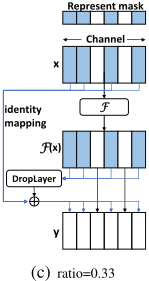
resent learning style (in Figure 1(b)) leads to a plain nonresidual network, which tends to progressively generate highlevel features but suffers from the degradation problem. By randomly configuring a certain ratio of channels to Represent learning style for each learning block, we obtain a network architecture which is good at generating new features and refining learnt features at the same time. Different from the dropout techniques that dynamically throw away part of the connections for each training sample or training batch, the channels without shortcut connections in each learning block are pre-configured randomly before the training. Therefore, randomness only occurs during the network configuration and all the training/testing samples are evaluated using the same network. Similar to HashedNet [Chen et al., 2015] and ShuffleNet [Zhang et al., 2017] which also pre-configure asymmetric networks, the feature learnt in each channel with RoR can adapt to the network architecture during the training.
The optimal ratio for feature channels in Represent learning style varies with different network architectures and applications. Intuitively, when more learning blocks are added, each individual learning block could take lower task loads on feature representation and the optimal ratio should be smaller; when the learning task is quite complex (though it is hard to measure task complexity in a quantitative manner), new features should be generated in deeper layers to capture highlevel concepts and hence a larger ratio is more beneficial. According to our experiments, a ratio around 0.05 works well for most conventional residual network architectures.
4 Experiments
We evaluate the performance of RoR using three image classification benchmarks: CIFAR-10, CIFAR-100 and ImageNet. We apply RoR on three conventional residual network architectures for image classification: ResNet, ResNeXt and SENet. During the famous ILSVRC Imagenet competition, the above three models have achieved the 1st place in 2015, the 2nd place in 2016 and the 1st place in 2017, respectively.
x
Represent mask
Channel
F
x
y
| Dataset | CIFAR10 | CIFAR100 | ImageNet |
|---|---|---|---|
| Resolution | 32×32 | 32×32 | 224×224 |
| #Train Images | 50K | 50K | 1280K |
| #Test Images | 10K | 10K | 50K |
| #Classes | 10 | 100 | 1000 |
| Model | #Params | #Blocks | Width | GFLOPs |
|---|---|---|---|---|
| ResNet-56 | 2.3M | 18 | 32 | 0.34 |
| ResNet-56s | 0.6M | 18 | 16 | 0.09 |
| ResNet-110 | 4.6M | 36 | 32 | 0.66 |
| ResNet-110s | 1.2M | 36 | 16 | 0.17 |
| ResNet-164 | 6.8M | 54 | 32 | 0.99 |
| ResNet-164s | 1.7M | 54 | 16 | 0.25 |
| ResNeXt-29 | 34.4M | 9 (x8) | 64 | 5.32 |
| ResNeXt-29s | 8.6M | 9 (x8) | 32 | 1.33 |
| SE-ResNeXt-29 | 34.4M | 9 (x8) | 64 | 5.33 |
| SE-ResNeXt-29s | 8.6M | 9 (x8) | 32 | 1.33 |
| ResNet-101 | 44.5M | 33 | 64 | 7.58 |
| ResNet-101s | 11.3M | 33 | 32 | 1.91 |
4.1 Experimental Setup
- Datasets. Table 1 summarizes the statistics of the three datasets. The resolution of images in CIFAR is 32×32, while all the images in ImageNet is pre-processed to a unified resolution 224×224. Standard data augmentation methods (mirroring+random shifting+cropping) are applied to CIFAR datasets. We apply the same data augmentation scheme described in [Szegedy et al., 2015] to ImageNet dataset. We also normalize the channel means to 0 and the channel standard deviations to 1 for all the datasets.
· Models for Comparison. Table 2 summarizes the details of residual learning models evaluated in the paper. ResNet56, ResNet-110 and ResNet-164 are the implementations of residual networks [He et al., 2016a] with 3-layer bottleneck learning blocks for CIFAR dataset. ResNet-101 is the implementation of residual networks for ImageNet as described in original paper. Since it takes much longer time to train models on ImageNet (e.g., ResNet-101 takes 7 days using 2 GTX Titan XP GPUs), we only conduct one group of comparison using ResNet-101 (i.e., 3×7 days) as the referred architecture. For the ResNeXt and SE-ResNeXt architectures with even larger model sizes and computational cost, we only evaluate their performance on CIFAR. ResNeXt-29 is the implementation of residual networks with aggregated group convolution [Xie et al., 2017] for CIFAR dataset, where the group cardinality is 8 and the base width within a group is 64. SEResNeXt-29 is the implementation of SE learning block [Hu et al., 2017] based on ResNeXt-29 for CIFAR dataset. For each of the models, we also implement a slim version where the feature channels are halved, and the parameter size and FLOPs are reduced by 4x, to further study the trade-off between performance and model complexity.
To evaluate the effectiveness of RoR, we replace the summation operation in each residual learning block of ResNet, ResNeXt and SENet with the RoR module proposed in this paper. For RoR module, we set Represent ratio to 0.05 and dropout rate to 0.2 by default in Section 4.2, and further study the effects of different parameter settings in Section 4.3 and 4.4. Residual learning with stochastic depth [Huang et al., 2016b] (SDepth) randomly drops the residual parts for each learning block. Since RoR also introduces the layer-level dropout operation to regularize the layer response, SDepth is exactly a special case of RoR where all channels are set to Refine learning style. Therefore, we also compare with SDepth, aiming to show the pure gain from explicit channel-wise learning rather than the advantages from simple regularization on the layer response.
| Model | Residual | SDepth | RoR |
|---|---|---|---|
| ResNet-56 | 6.43 | 5.76 | 4.79 |
| ResNet-56s | 7.17 | 6.85 | 6.17 |
| ResNet-110 | 5.91 | 5.39 | 4.66 |
| ResNet-110s | 6.68 | 5.93 | 5.48 |
| ResNet-164 | 5.41 | 4.78 | 4.54 |
| ResNet-164s | 6.52 | 5.25 | 4.84 |
| ResNeXt-29 | 3.65 | 3.85 | 3.72 |
| ResNeXt-29s | 4.35 | 4.36 | 4.28 |
| SE-ResNeXt-29 | 3.83 | 3.91 | 3.45 |
| SE-ResNeXt-29s | 4.28 | 4.26 | 4.33 |
| Model | Residual | SDepth | RoR |
|---|---|---|---|
| ResNet-56 | 26.95 | 27.02 | 23.93 |
| ResNet-56s | 29.75 | 29.16 | 27.14 |
| ResNet-110 | 25.10 | 24.31 | 22.77 |
| ResNet-110s | 28.79 | 27.45 | 26.35 |
| ResNet-164 | 23.18 | 22.68 | 21.58 |
| ResNet-164s | 27.76 | 24.98 | 24.18 |
| ResNeXt-29 | 17.77 | 17.98 | 17.05 |
| ResNeXt-29s | 19.43 | 19.41 | 18.55 |
| SE-ResNeXt-29 | 17.72 | 17.83 | 17.12 |
| SE-ResNeXt-29s | 19.35 | 19.53 | 18.73 |
| Model | Residual | SDepth | RoR |
|---|---|---|---|
| ResNet-101 | 21.78 | 21.98 | 21.15 |
| ResNet-101s | 24.33 | 24.11 | 23.38 |
- Implementation and Training. All the models are implemented using PyTorch and trained with 2 GTX Titan XP GPUs. We train models on CIFAR dataset for 300 epochs and models on ImageNet dataset for 80 epochs. For all the models, standard mini-batch SGD with momentum is used as the optimization method. The batch size is set to 128 and momentum is set to 0.9. All the parameters are initialized using the method described in [He et al., 2015]. The learning rate starts from 0.01 and is reduced by 10x when 50% and 75% of the epochs are finished. The top-1 accuracy on test dataset is evaluated at termination.
4.2 Comparison Results
We provide the error rates of different models on CIFAR datasets in Table 3 and 4. For CIFAR10, our RoR models outperform all the original residual networks with different depths, achieving error rates of 4.79%, 4.66% and 4.54% on ResNet-56, ResNet-110 and ResNet-164, respectively. Remarkably, the slim versions of RoR models, using only half of the feature channels, 1/4 parameter size and computation cost, achieve lower error rates than the non-slim ResNets in all the depths. RoR also performs better than ResNets with SDepth by reducing the error rate by 7%-16%. The performance of RoR is slightly behind, but still comparable to the two advanced ResNets variants: ResNeXt and SE-ResNeXt. This may be explained by that CIFAR10 is a relatively easy task and the usage of ResNeXt is an overkill that there is no need to further increase its ability of represent new features by introducing RoR blocks.
More encouraging results are observed on CIFAR100: the models with RoR blocks perform consistently better than the the original ResNets and those with SDepth. Compared with ResNets, RoR reduces error rate by over 10% for all the network depths. RoR outperforms ResNeXt and SE-ResNeXt by reporting 2.5% and 2.3% lower error rates, respectively.
We report the results on ImageNet in Table 5. RoR suppresses the original ResNets and the one with SDepth, by reducing 0.6% and 0.8% error rates, respectively. The advantage of RoR on the slim version becomes more significant, i.e., slim RoR achieves 1.0% lower error rate than slim ResNets. All these results reveal the effectiveness of RoR with fine-grained channel-wise configuration on complex classification tasks.
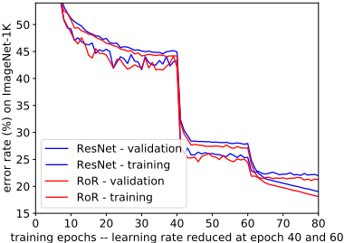
Figure 2 depicts the training and validation curves on ImageNet. The trends are consistent to the results in Table 5. RoR achieves lower error rates than ResNets on both training and validation datasets. Notice that training RoR models is also efficient as no extra parameters are introduced, compared with the training of the plain residual networks.
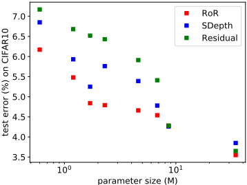
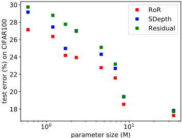
Figure 3 and Figure 4 show the parameter efficiency of RoR, SDepth and ResNets on two CIFAR datasets, respectively. We can see that RoR is consistently the most parameter efficient model, mainly because it allows the emergence of new features in each learning block. To achieve the same level of accuracy, RoR requires much smaller number of parameters than both SDepth and ResNets, e.g., RoR uses less than 1/5 of the parameters of SDepth and ResNets for achieving 5.55% test error.
4.3 Effect of Represent Channels
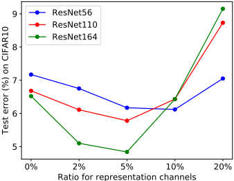
We now assess the effect of Represent channels on RoR models. From Figure 5, we observe that the test error on CIFAR10 using RoR exhibits a U-shape curve by varying the ratio of Represent channels. Similar results are observed on other datasets and we omit the figures due to page limit. For each of the three ResNets with RoR blocks, the lowest error rate is achieved by using a moderate ratio of Represent channels, i.e., 5%. The models with smaller ratios have more Refine channels and hence the performance will be degraded to that of the plain ResNets. The advantages of deeper structures with plain residual learning blocks become less significant, which can be indicated by the similar test errors from ResNets in different depths using a ratio of 0. However, it is important to note that RoR reduces error significantly on deeper network structures by using 5% Represent channels. This verifies the effectiveness of Represent channels on deeper model learning. As the ratio becomes larger, the error rate reported by RoR increases, especially on deeper models. This is reasonable as CIFAR10 is a simple classification task and more Represent channels will cause the overfitting problem.
4.4 Effect of Regularization
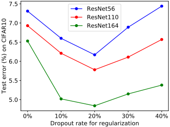
We next investigate the effect of regularization on Refine channels. Figure 6 shows the error rates by varying dropout rate for regularization. We make the following three observations. First, DropLayer for Refine channels will benefit model performance and RoR models in different depths consistently achieve the lowest error rates when the dropout rate is set to 20%. Second, dropout rate is not a dominant factor to model performance and the performance gain of RoR models always benefits from deeper model structures when the dropout rate varies from 0 to 40%. Finally, relatively larger dropout rates (e.g., 40%) achieve better performance than smaller rates (e.g., 0), which follows our intuition that the refined features should be closer to the original basic ones.
5 Conclusion
In this paper, we propose a novel Refine or Represent (RoR) module to distinguish the learning style on channel basis. We define two types of channel-wise learning styles, where channels in Refine style are learned via the conventional residual function with a regularization on the channel response, and those in Represent style act as plain learning blocks for feature representation. We adopt a random scheme to deploy explicit learning style configuration for each channel. Our RoR module can be easily applied to a range of residual learning blocks, without introducing extra model parameters. Extensive experiments on CIFAR and ImageNet benchmark tasks demonstrate the effectiveness of RoR module in terms of accuracy and parameter efficiency.
Acknowledgments
This work is supported in part by National Research Foundation, Prime Ministers Office, Singapore under CRP Award No. NRF-CRP8-2011-08, and NSFC (No. 61602297).
@inproceedings{ijcai2018p372,
  title     = {Refine or Represent: Residual Networks with Explicit Channel-wise Configuration},
  author    = {Shen, Yanyan and Gao, Jinyang},
  booktitle = {Proceedings of the Twenty-Seventh International Joint Conference on
               Artificial Intelligence, {IJCAI-18}},
  publisher = {International Joint Conferences on Artificial Intelligence Organization},
  editor    = {Jérôme Lang},
  pages     = {2682--2688},
  year      = {2018},
  month     = {7},
  note      = {Main track},
  doi       = {10.24963/ijcai.2018/372},
  url       = {https://doi.org/10.24963/ijcai.2018/372},
}
TY - CPAPER TI - Refine or Represent: Residual Networks with Explicit Channel-wise Configuration AU - Shen, Yanyan AU - Gao, Jinyang T2 - Proceedings of the Twenty-Seventh International Joint Conference on Artificial Intelligence, IJCAI-18 PB - International Joint Conferences on Artificial Intelligence Organization PY - 2018 SP - 2682 EP - 2688 DO - 10.24963/ijcai.2018/372 UR - https://doi.org/10.24963/ijcai.2018/372 ER -Copied
Machine-readable versions of this paper, for tools and AI agents:





