
Deep Discrete Prototype Multilabel Learning
Proceedings of the Twenty-Seventh International Joint Conference on Artificial Intelligence. Main track. Pages 2675-2681.
https://doi.org/10.24963/ijcai.2018/371
Keywords
- Machine Learning: Classification
- Machine Learning: Multi-instance;Multi-label;Multi-view learning
Abstract
kNN embedding methods, such as the state-of-the-art LM-kNN, have shown impressive results in multi-label learning. Unfortunately, these approaches suffer expensive computation and memory costs in large-scale settings. To fill this gap, this paper proposes a novel deep prototype compression, i.e., DBPC for fast multi-label prediction. DBPC compresses the database into a small set of short discrete prototypes, and uses the prototypes for prediction. The benefit of DBPC comes from two aspects: 1) The number of distance comparisons are reduced in the prototype; 2) The distance computation cost is significantly decreased in the reduced space. We propose to jointly learn the deep latent subspace and discrete prototypes within one framework. The encoding and decoding neural networks are employed to make deep discrete prototypes well represent the instances and labels. Extensive experiments on several large-scale datasets demonstrate that DBPC achieves several orders of magnitude lower storage and prediction complexity than state-of-the-art multi-label methods, while achieving competitive accuracy.
- [Bhatia et al., 2015] Kush Bhatia, Himanshu Jain, Purushot- tam Kar, Manik Varma, and Prateek Jain. Sparse local em- beddings for extreme multi-label classification. In NIPS, pages 730-738, 2015.
- [Chatfield et al., 2014] Ken Chatfield, Karen Simonyan, An- drea Vedaldi, and Andrew Zisserman. Return of the devil in the details: Delving deep into convolutional nets. In BMVC, 2014.
- [Chen and Lin, 2012] Yao-Nan Chen and Hsuan-Tien Lin. Feature-aware label space dimension reduction for multi- label classification. In NIPS, pages 1529-1537, 2012.
- [Chua et al., 2009] Tat-Seng Chua, Jinhui Tang, Richang Hong, Haojie Li, Zhiping Luo, and Yantao Zheng. Nus- wide: a real-world web image database from national uni- versity of singapore. In CIVR, 2009.
- [Cissé et al., 2016] Moustapha Cissé, Maruan Al-Shedivat, and Samy Bengio. ADIOS: architectures deep in output space. In ICML, pages 2770-2779, 2016.
- [Fan et al., 2008] Rong-En Fan, Kai-Wei Chang, Cho-Jui H- sieh, Xiang-Rui Wang, and Chih-Jen Lin. Liblinear: A library for large linear classification. JMLR, 9:1871-1874, 2008.
- [García et al., 2012] Salvador García, Joaquín Derrac, José Ramón Cano, and Francisco Herrera. Prototype selection for nearest neighbor classification: Taxonomy and empirical study. 34(3):417-435, 2012.
- [Hsu et al., 2009] Daniel Hsu, Sham Kakade, John Lang- ford, and Tong Zhang. Multi-label prediction via com- pressed sensing. In NIPS, pages 772-780, 2009.
- [Kusner et al., 2014] Matt J. Kusner, Stephen Tyree, Kil- ian Q. Weinberger, and Kunal Agrawal. Stochastic neigh- bor compression. In ICML, pages 622-630, 2014.
- [Kwok and Tsang, 2003] James T. Kwok and Ivor W. Tsang. Learning with idealized kernels. In ICML, pages 400-407, 2003.
- [Liu and Tsang, 2015] Weiwei Liu and Ivor W. Tsang. Large margin metric learning for multi-label prediction. In AAAI, pages 2800-2806, 2015.
- [Liu and Tsang, 2017] Weiwei Liu and Ivor W. Tsang. Mak- ing decision trees feasible in ultrahigh feature and label dimensions. JMLR, 18:81:1-81:36, 2017.
- [Liu et al., 2017] Weiwei Liu, Ivor W. Tsang, and Klaus- Robert Müller. An easy-to-hard learning paradigm for multiple classes and multiple labels. JMLR, 18:94:1- 94:38, 2017.
- [Nam et al., 2017] Jinseok Nam, Eneldo Loza Mencía, Hyunwoo J. Kim, and Johannes Fürnkranz. Maximizing subset accuracy with recurrent neural networks in multi- label classification. In NIPS, pages 5419-5429, 2017.
- [Norouzi et al., 2012] Mohammad Norouzi, David J. Fleet, and Ruslan Salakhutdinov. Hamming distance metric learning. In NIPS, pages 1070-1078, 2012.
- [Schönemann, 1966] Peter H Schönemann. A generalized solution of the orthogonal procrustes problem. Psychome- trika, 31(1):1-10, 1966.
- [Shen et al., 2017] Xiaobo Shen, Weiwei Liu, Ivor W. Tsang, Fumin Shen, and Quan-Sen Sun. Compressed k-means for large-scale clustering. In AAAI, pages 2527-2533, 2017.
- [Shen et al., 2018] Xiaobo Shen, Weiwei Liu, Ivor W. Tsang, Quan-Sen Sun, and Yew-Soon Ong. Multilabel prediction via cross-view search. TNNLS, PP(P):1-15, 2018.
- [Tai and Lin, 2012] Farbound Tai and Hsuan-Tien Lin. Mul- tilabel classification with principal label space transforma- tion. Neural Computation, 24(9):2508-2542, 2012.
- [Tsoumakas et al., 2009] Grigorios Tsoumakas, Ioannis Katakis, and Ioannis Vlahavas. Mining multi-label data. In Data mining and knowledge discovery handbook, pages 667-685. 2009.
- [Wang et al., 2018] Jingdong Wang, Ting Zhang, Jingkuan Song, Nicu Sebe, and Heng Tao Shen. A survey on learn- ing to hash. TPAMI, 40(4):769-790, 2018.
- [Xu et al., 2015] Zhixiang Eddie Xu, Jacob R. Gardner, Stephen Tyree, and Kilian Q. Weinberger. Compressed support vector machines. CoRR, abs/1501.06478, 2015.
- [Zhang and Schneider, 2011] Yi Zhang and Jeff Schneider. Multi-label output codes using canonical correlation anal- ysis. In AISTATS, pages 873-882, 2011.
- [Zhang and Schneider, 2012] Yi Zhang and Jeff Schneider. Maximum margin output coding. In ICML, pages 1575- 1582, 2012.
- [Zhang and Zhou, 2007] Min-Ling Zhang and Zhi-Hua Zhou. ML-KNN: A lazy learning approach to multi-label learning. PR, 40(7):2038-2048, 2007.
- [Zhang and Zhou, 2014] Min-Ling Zhang and Zhi-Hua Zhou. A review on multi-label learning algorithms. TKDE, 26(8):1819-1837, 2014.
- [Zhang et al., 2009] Kai Zhang, James T. Kwok, and Bahram Parvin. Prototype vector machine for large scale semi-supervised learning. In ICML, pages 1233-1240, 2009.
- [Zhong et al., 2017] Kai Zhong, Ruiqi Guo, Sanjiv Kumar, Bowei Yan, David Simcha, and Inderjit S. Dhillon. Fast classification with binary prototypes. In AISTATS, pages 1255-1263, 2017.
References were extracted automatically from the PDF and may contain errors.
Full text extracted automatically from the PDF; figures, tables and equations may differ. The PDF is the version of record.
1 Introduction
In multi-label learning [Tsoumakas et al., 2009; Chen and Lin, 2012; Zhang and Zhou, 2014; Bhatia et al., 2015; Liu and Tsang, 2017; Liu et al., 2017; Shen et al., 2018], each instance is represented by a set of labels. For example, a document can be associated with a range of topics, such as sports, finance, and education; or an image may be tagged with both beach and tree. The task of multi-label learning is to learn a function that can predict the proper label sets for unseen instances. Nowadays, it plays a vital role in a number of applications, ranging from document classification to gene function prediction and automatic image annotation.
Hsu et al. [2009] first propose to embed the label space into a low-dimensional subspace using random projection, and then build a regression model in the embedding space. To learn better embeddings, various embedding methods have since been developed, such as canonical correlation analysis (CCA) [Zhang and Schneider, 2011], maximum margin output coding (MMOC) [Zhang and Schneider, 2012]. Such methods have achieved the impressive performance on small datasets. However, their decoding schemes often require solving a quadratic programming (QP) problem in a combinatorial space, which is not tractable even for medium-sized datasets.
∗Corresponding author.
K nearest neighborhood (kNN) technique is attractive in multi-label learning due to its simplicity and interpretability. Comprehensive researches show that kNN achieves very competitive performances when handling many labels and classes [Bhatia et al., 2015]. Multi-label KNN (ML-KNN) [Zhang and Zhou, 2007] is the first work that applies kNN into multi-label prediction. ML-KNN finds the k nearest neighbors in the training datasets, and uses the maximum posteriori principle for prediction. Inspired by the fact that the prediction performance of kNN can be greatly improved by learning a specific distance metric [Kwok and Tsang, 2003], large margin kNN (LM-kNN) [Liu and Tsang, 2015] has been proposed. LM-kNN learns a distance metric to discover the label dependency such that instances with very different multiple labels are moved further away. LM-kNN employs kNN search in the learned embedding space to further improve the efficiency of prediction. Another state-of-the-art method that also uses kNN search for fast prediction is the recently proposed sparse local embedding for extreme classification (SLEEC) [Bhatia et al., 2015]. SLEEC first seeks the embedding of labels by preserving the pairwise distances between a few nearest label neighbors, and then learns the regressor in the embedding space. The computational complexity of kNN is O(nd), where n and d are the size of database and the dimensionality of embedding space. Thus, these methods are computationally very expensive on large-scale datasets. Besides, kNN stores the entire embeddings of the database in memory, which is also prohibitive in resource constrained devices, e.g., cellphone. How to relieve the computation and storage costs of kNN in large-scale multi-label prediction remains less explored.
Prototype learning is an economical way to improve the scalability and efficiency of the learning models, e.g., kNN classification [Garc´ıa et al., 2012; Kusner et al., 2014; Zhong et al., 2017], semi-supervised learning (SSL) [Zhang et al., 2009], support vector machine [Xu et al., 2015]. Prototype vector machine (PVM) [Zhang et al., 2009] uses prototypes to efficiently approximate both graph-based regularizer and model representation. A small set of prototypes in kNN classification can be also used to replace the whole database, and a testing instance is only compared within this small set. Thus, the prediction time is dramatically reduced. The idea behind prototype is that the redundant instances can be removed to reduce the prediction complexity [Garc´ıa et al., 2012]. Stochastic neighbor compression (SNC) [Kusner et al., 2014] is recently proposed to compress data for fast kNN classification. SNC learns the prototypes by minimizing the kNN training classification error on them.
Binary code learning [Wang et al., 2018] has gained increased interests in many large-scale applications. The basic idea of binary code learning is to encode the original highdimensional data into a set of short binary codes with similarity preservation. The advantage of binary coding is that it can perform an effective search in Hamming space at very low cost of both storage and computation. Many binary code learning methods [Wang et al., 2018; Norouzi et al., 2012; Shen et al., 2017] have been developed to facilitate largescale applications.
Inspired by the great success of the prototype and binary code learning in large-scale applications, this paper proposes a new technique, dubbed deep binary prototype compression (DBPC) for fast multi-label prediction. DPBC simultaneously learns binary prototypes and hash function, such that a testing instance is first mapped into the Hamming space by hash function, and then matches with a small set of binary prototypes for prediction. Moreover, the encoding and decoding neural networks are employed to enable the prototypes to discover the latent nonlinear structure among the data. The advantages of DBPC lie in the low cost of storage and prediction complexity. Taking the MIRFLICKR25K dataset as an example, DPBC reduces the storage of kNN around 20480 times from 520MB to 26KB; meanwhile, the prediction time of DPBC is 5.63s, which is nearly 146 times faster than kNN. The main contributions of this work are summarized below:
- We propose a new multi-label prediction method, named deep binary prototype learning (DBPC), which compresses the whole database into a small set of binary prototypes. DBPC can achieve the low storage and complexity cost.
- The proposed DBPC is formulated to jointly learn the deep latent hamming space and binary prototypes within a unified framework. The encoding and decoding neural networks are employed to make deep binary prototypes well represent the instances and labels.
- Extensive experiments on several large-scale datasets demonstrate that DBPC obtains several orders of magnitude lower storage and prediction complexity than stateof-the-art multi-label methods, while achieving satisfactory accuracy.
The organization of this paper is arranged as follows. In Sections 2, we discuss KNN embedding methods for multilabel prediction. Section 3 introduces deep binary prototype compression method. The experiment is presented in Section 4, and the conclusion is drawn in Section 5.
2 KNN EmbeddingMethods for Multi-label Prediction
Let {(xi, yi)}ni=1 be the training dataset, xi ∈ X ⊆ Rp be an input (instance) vector, yi ∈ V ⊆ {0, 1}q be the corresponding output (label) vector, and let n denote the number of training instances. || · ||F and || · ||1 represent the Frobenius norm and l1 norm, respectively. Let X = [x1, x2, . . . , xn] ∈ Rp×n be the instance matrix and Y = [y1, y2, . . . , yn] ∈ Rq×n be the label matrix. The goal of multi-label learning is to learn a model that accurately predicts the label vector for testing instances.
Embedding methods aim to learn a function f : Rp → Rd (d < p) to map any instance into a low-dimensional subspace Z. Given a testing instance x, its k nearest neighbors are searched in Z, and kNN prediction function for multi-label learning is defined as
where ˆy is the predicted label vector of x. ρ is the round function, i.e., ρ(y) equals 1 if y ≥ t holds, and 0 otherwise, t is a predefined threshold, which is set to 0.5 in this work. 1 is the indicator function, i.e., 1[π] equals 1 if π holds and 0 otherwise. Nk(z) is the set of k nearest neighbors of z in Z, z and zi are the embeddings of x and xi respectively.
The computational complexity is O(nd) for predicting a testing instance in (1). If n is large, it will be computationally expensive even with a medium-length d. Besides, kNN stores the entire embedding of X in memory, which is also prohibitive in resource constrained devices. A challenging problem is how to efficiently perform kNN search for multilabel prediction on large-scale datasets. In the following sections, we introduce the binary prototype technique to address the above issues.
3 Deep Binary Prototype Compression
3.1 Binary Prototype KNNDecision Rule
We propose to use a small set of binary prototypes to represent the entire training set. Specifically, our goal is to find a low-dimensional hamming space B, and m binary prototypes B = [b1, b2, . . . , bm] ∈ {-1, 1}d×m (m ≪ n), with the corresponding label vectors, i.e., V = [v1, v2, . . . , vm] ∈ Rq×m, such that the label vector of any testing instance can be accurately predicted using kNN search on the prototypes. We further define the hash function f : Rp → {-1, 1}d to map instances into Hamming space.
Given the above definitions, we present the binary prototype kNN prediction function in B
Algorithm 1 Binary Prototype KNN Prediction
Input: Testing instance: x, number of NN: k, hash function: f, binary prototype: B, prototype label vector: V. Output: ˜ y.
- 1: Compute the binary embedding of x, b = sgn(f(x));
- 2: Obtain the set Nk(b) by finding the k nearest binary prototype neighbors of x in B;
- 3: Predict the label vector ˜ y via (2).
where b is the binary code of the given input x, i.e., b = sign (f(x)), bi is the i-th prototype in B, Nk(b) is the set of k nearest binary prototype neighbors of b. For simplicity, we fix the prototypes V by performing k-means clustering on Y. The multi-label prediction via kNN search on binary prototypes is illustrated in Algorithm 1.
Compared with the conventional kNN prediction rule defined in (1), (2) improves the prediction efficiency in two aspects: 1) kNN search in (2) only goes through a small set of prototypes, thus the number of distance computation can be greatly reduced; 2) As the prototypes are binary, distance computation is very fast using the Hamming metric.
3.2 Formulation
Existing methods, such as SLEEC and LM-kNN, employ a linear transformation between the input and embedding spaces. Linear model may not capture the underlying data distribution. Inspired by recent advance in deep learning, we propose a new method, dubbed Deep Binary Prototype Compression (DBPC), to learn the nonlinear prototypes via deep neural network (NN).
Specifically, DBPC comprises encoding NN f : Rp → {-1, 1}d to map instance into Hamming space, and decoding NN g : {-1, 1}d → Rq to map Hamming space to label space. DBPC minimizes the following objective function
The constraint enforces the embeddings to be binary. We further propose to approximate any binary embedding in training set via its nearest binary prototype. For the i-th instance, we have
where hi ∈ {0, 1}m×1 is the indicator vector, and ‖hi‖1 = 1, which indicates only one entry in hi equals 1 and all the others equal 0. hi aims to select the nearest prototype for the i-th instance. The indicator matrix is defined as H = [h1, h2, . . . , hn] ∈ {0, 1}m×n , which can be obtained by matching V and Y.By substituting (4) into (3), we have
By applying the quadratic penalty method, we minimize the following objective function
where µ is a nonnegative regularization parameter. It can be further rewritten as a compact form
where the constraint BB⊤ = mId is introduced to make d bits mutually uncorrelated, such that the redundancy among these bits can be minimized, and Id represents an d × d identity matrix.
Generally, (7) is difficult to solve because of the binary constraint. We first define a set Ω = {Z ∈ Rd×m|ZZ⊤ = mId}, and then provide a new formulation that softens the orthogonal constraint in (7) as
where dist (B, Ω) = minZ∈Ω ‖B - Z‖F measures the distance from B to the set Ω, and α ≥ 0 is a regularization parameter. In (8), we allow a certain discrepancy between B and Ω, such that (8) is more flexible than (7).
3.3 Optimization
We design a tractable alternating optimization algorithm to iteratively optimize each variable. The flowchart of DBPC is described by Algorithm 2.
1) f, g Step Given B, we use back-propagation (BP) with mini-batch gradient descent method to update the parameters of both encoding and decoding NNs. The outputs of encoding and decoding NNs are represented as F = f(X) and G = g(BH) respectively. We compute the gradient of L with respect to F as follows
Besides, the gradient of L with respect to G can be similarly obtained
Then the chain rule is applied to update the network parameters of f and g.
2) B Step Given f, g, and Z, the sub-problem with respect to B can be reduced to
Algorithm 2 Deep Binary Prototype Compression
Input: training dataset: {(xi, yi)}ni=1 , binary prototype size: m, embedding dimensionality: d, parameter: µ, α, iteration number: T.
Output: NNs: f, g, binary prototypes: B.
- 1: Obtain V, H by performing k-means on Y.
- 2: Initialize Z by performing PCA on V.
- 3: Initialize B= sgn (Z).
- 4: repeat
- 5: for i = 1 → T do
- 6: Forward to compute F in a mini-batch;
- 7: Calculate the derivation according to (9);
- 8: Update the parameters in encoding NN f by using back propagation.
- 9: end for
- 10: for i = 1 → T do
- 11: Forward to compute G in a mini-batch;
- 12: Calculate the derivation according to (10);
- 13: Update the parameters in decoding NN g by using back propagation.
- 14: end for
- 15: Update B via (13) iteratively;
- 16: Compute SVD decomposition of B, B= PΣQ⊤;
- 17: Update Z as Z = √mPQ⊤;
- 18: until converge or reach maximum iterations
where G= g(BH). (11) involves the binary constraint, thus it is very challenging, and has no closed-form solution. Inspired by the recent advance in nonconvex optimization, we propose to optimize (11) with proximal gradient method. The main idea is to iteratively optimize a surrogate function. In specific, we iteratively optimize a local function ˆ Li(B) that linearizes L(B) at the point B(i) , and employ ˆ Li(B) as a surrogate of L(B). Given B(i) , the next discrete point B(i+1) can be derived by optimizing the following objective function
where τ > 0 is a constant, ∇L(B(i) ) = ∇1H⊤ - µFH⊤ - αZ, ∇1 is the gradient with respect to the input of the 1th layer in g. ∇1 can be calculated via the chain rule, and the gradient with respect to G(i) is set to (G(i) -Y), where G(i) = g(B(i)H). Then the updating rule for B(i+1) can be defined as
where sgn is the sign function, the function C (x, y) = {x, x ̸= 0 y, x = 0 , C is applied in an element-wise manner in (13) to eliminate the zero entries.
- Z Step The sub-problem with respect to Z is defined as follows
| Datasets | #Instances | #Features | #Labels | #Card-Label |
|---|---|---|---|---|
| DELICIOUS | 16,105 | 500 | 983 | 19.020 |
| EUR-LEX | 19,348 | 5,000 | 3,993 | 1.292 |
| MIRFLICKR25K | 25,000 | 224×224 | 24 | 3.716 |
| NUS-WIDE | 161,788 | 224×224 | 81 | 1.869 |
Although there is a non-convex constraint on Z, we fortunately show that (14) admits a closed-form solution. The closed-form solution of (14) can be characterized by the following theorem.
Theorem 1. The singular value decomposition (SVD) of B is defined as B = PΣQ⊤, Σ is a diagonal matrix containing the singular values, P and Q are left and right singular matrices respectively. Z = √mPQ⊤ is an optimal solution to optimization problem in (14).
Proof. (14) is the classic Orthogonal Procrustes problem. The proof of this theorem can be adapted from [Sch¨onemann, 1966].
3.4 Computational Complexity Analysis
We first analyze the computational complexity of prediction in the proposed DPBC. Given a testing instance x, it takes O(ζm) for prediction, where O(ζ) denotes the computational complexity for d-bit calculations. Existing kNN and kNN embedding methods require O(pn) and O(dn) for prediction. Due to the reduced number of comparisons and computation costs in Hamming space, DBPC is obviously efficient in prediction.
In terms of space complexity, DBPC only needs to store the binary prototypes B, which counts for O(dm) bits. The existing kNN and kNN embedding methods needs to store O(pn) and O(dn) real-valued numbers. Given m ≪ n, d < p, DBPC has much lower space complexity than existing network embedding methods.
4 Experiments
In this section, we evaluate the performance of the proposed method for multi-label classification. All the experiments are performed on a Ubuntu 64-Bit Linux workstation with 24core Intel Xeon CPU E5-2620 2.10 GHz and 128 GB memory.
4.1 Experimental Setup
Datasets The experiments are conducted on four real-world multi-label datasets, whose statistics are summarized in Table 1.
- DELICIOUS 1 : contains textual data of web pages along with 983 tags extracted from the del.icio.us social book marking site. 3-fold cross-validation is applied to split training and testing sets.
- EUR-Lex1 : collects documents on European Union law. There are several EuroVoc descriptors, directory codes and types of subject matter to describe the labels. Here,
1 http://mulan.sourceforge.net
| Datasets | Example-F1 ↑ | ||||||
|---|---|---|---|---|---|---|---|
| BR | PLST | kNN | ML-kNN | LM-kNN | SLEEC | DBPC | |
| DELICIOUS | .2091 ± .0079 | .1021 ± .0078 | .1641 ± .0057 | .1494 ± .0047 | .2345 ± .0061 | .2024 ± .0026 | .2552 ± .0058 |
| EUR-LEX | .3619 ± .0087 | .0972 ± .0089 | .3138 ± .0032 | .2701 ± .0064 | .3445 ± .0050 | .3343 ± .0050 | .3516 ± .0069 |
| MIRFLICKR25K | .5329 ± .0063 | .5062 ± .0082 | .5624 ± .0058 | .5557 ± .0042 | .6035 ± .0059 | .6212 ± .0075 | .6429 ± .0062 |
| NUS-WIDE | .512 | .479 | .504 | .529 | .552 | .625 | .637 |
| Micro-F1 ↑ | |||||||
| Datasets | BR | PLST | kNN | ML-kNN | LM-kNN | SLEEC | DBPC |
| DELICIOUS | .2420 ± .0042 | .1323 ± .0048 | .1916 ± .0061 | .1704 ± .0052 | .2862 ± .0078 | .2383 ± .0051 | .2768 ± .0041 |
| EUR-LEX | .3965 ± .0073 | .1247 ± .0093 | .3757 ± .0078 | .3168 ± .0067 | .4026 ± .0068 | .3883 ± .0049 | .4269 ± .0050 |
| MIRFLICKR25K | .5833 ± .0068 | .5864 ± .0089 | .6232 ± .0072 | .6080 ± .0069 | .6531 ± .0061 | .6773 ± .0062 | .6992 ± .0068 |
| NUS-WIDE | .535 | .483 | .529 | .546 | .576 | .643 | .664 |
| Macro-F1 ↑ | |||||||
| Datasets | BR | PLST | kNN | ML-kNN | LM-kNN | SLEEC | DBPC |
| DELICIOUS | .0854 ± .0057 | .0295 ± .0042 | .0502 ± .0012 | .0463 ± .0011 | .1236 ± .0078 | .0632 ± .0015 | .1165 ± .0036 |
| EUR-LEX | .0982 ± .0075 | .0502 ± .0042 | .0935 ± .0025 | .0591 ± .0014 | .0987 ± .0029 | .0725 ± .0025 | .1145 ± .0035 |
| MIRFLICKR25K | .5042 ± .0035 | .2532 ± .0067 | .4627 ± .0075 | .4590 ± .0081 | .5326 ± .0071 | .5511 ± .0086 | .5839 ± .0062 |
| NUS-WIDE | .332 | .269 | .346 | .356 | .364 | .467 | .493 |
we use one of them which has more labels. 3-fold crossvalidation is applied to split training and testing sets.
- MIRFLICKR25K 2 : consists of 25,000 images collected from the social photography website Flickr. All images are annotated for 24 semantic concepts including various scenes and objects categories such as sky, night, food, and tree. All the images are resized to 224×224. 3-fold cross-validation is applied to split training and testing sets.
- NUS-WIDE 3 : consists of 269,648 images from 81 ground-truth concepts with a total number of 5,018 unique tags. All the images are resized to 224×224. Followed by the publicly available experimental setting [Chua et al., 2009], we select 161,789 samples as the training set, and the remaining 107,859 samples as the testing set.
Experimental Setting We compare the proposed method with seven state-of-the-art multi-label learning methods, i.e., BR [Tsoumakas et al., 2009], PLST [Tai and Lin, 2012], kNN, ML-kNN [Zhang and Zhou, 2007], LM-kNN [Liu and Tsang, 2015], and SLEEC [Bhatia et al., 2015]. The linear classification/regression package LIBLINEAR [Fan et al., 2008] with ℓ2-regualrized logistic regression is adopted to train the classifier for BR. Following the experimental settings [Liu and Tsang, 2015], we set η = 0.4 in LM-kNN, and C = 10 in BR and LM-kNN. According to the original settings [Bhatia et al., 2015], we set the number of the clusters to ⌊n/6000⌋ and the number of learners to 15 for SLEEC, where ⌊δ⌋ is the greatest integer less than or equal to δ. Following the similar settings in [Zhang and Zhou, 2007; Bhatia et al., 2015], the k in kNN search is determined using 5-fold cross validation over the range {1, 5, 10, 20} for all kNN-based methods. The dimension of the embedding in SLEEC and DBPC is set to 128 for all the datasets.
2 http://press.liacs.nl/mirflickr/
3 http://lms.comp.nus.edu.sg/research/NUS-WIDE.htm
For the non-deep comparison methods, we use 4,096dimensional deep features of MIRFLICKR25K and NUSWIDE extracted by the pre-trained CNN-F model [Chatfield et al., 2014] for fair comparison. Both encoding and decoding NNs in our proposed DBPC consist two fully-connected layers on DELICIOUS and EUR-LEX datasets, where the first layer has 4,096 nodes. For MIRFLICKR25K and NUSWIDE, encoding NN has eight layers, where the first seven layers are adopted from CNN-F model [Chatfield et al., 2014], and the eighth layer is a fully-connected layer. The activation functions for the previous and last layers are ReLU and identity functions, respectively. We fix the mini-batch size to 128 and tune the learning rate from 10-6 to 10-2 by cross validation; µ and α are set to 0.1 and 0.01 respectively; τ is selected from [1, 10] by cross validation. We set the size of prototype set in DBPC as ⌊n ∗ ρ⌋, where ratio ρ is set to 0.1 in this work.
EvaluationMetric Following [Liu and Tsang, 2015; Bhatia et al., 2015], we consider the widely-used metrics to evaluate the prediction performance of all the methods, i.e., ExampleF1, Micro-F1, Macro-F1. In addition, we also conduct the comparisons in terms of prediction computation and memory costs.
4.2 Performance
We conduct the performance evaluation on four multi-label datasets. Table 2 reports the prediction results of all the methods, in terms of Example-F1, Micro-F1, Macro-F1. From Table 2, we observe that 1) The proposed DBPC generally achieves the best performance on four datasets. For example, on MIRFLICKR25K, in terms of Example-F1, Micro-F1, Macro-F1, DBPC improves the best results of the baselines by 2.12%, 2.19%, 3.28%, respectively. The above results demonstrate the superior performance of the proposed DBPC. 2) Among kNN-based baselines, LM-kNN and SLEEC obtain the better performance, which are consistent with the empirical results in [Liu and Tsang, 2015] and [Bhatia et al., 2015].
| Dataset | kNN | ML-kNN | LM-kNN | SLEEC | DBPC Time(s) | ||||
|---|---|---|---|---|---|---|---|---|---|
| Time(s) | Speedup | Time(s) | Speedup | Time(s) | Speedup | Time(s) | Speedup | ||
| DELICIOUS | 46.61 | 41× | 63.01 | 53× | 84.67 | 75× | 28.10 | 25× | 1.13 |
| EUR-LEX | 648.21 | 316× | 107.97 | 52× | 105.36 | 51× | 30.57 | 15× | 2.05 |
| MIRFLICKR25K | 823.95 | 146× | 91.26 | 16× | 425.86 | 75× | 123.29 | 22× | 5.63 |
| NUS-WIDE | 3.59 ×10⁴ | 36× | 5.53 ×10⁴ | 56× | 7.81 ×10³ | 8× | 4.09 ×10³ | 4× | 978 |
| Dataset | kNN | SLEEC | DBPC | ||
|---|---|---|---|---|---|
| Mem. | Red. | Mem. | Red. | Mem. | |
| DELICIOUS | 41MB | 2500× | 10MB | 640× | 17KB |
| EUR-LEX | 492MB | 25000× | 12MB | 640× | 20KB |
| MIRFLICKR25K | 520MB | 20480× | 16MB | 640× | 26KB |
| NUS-WIDE | 4.94GB | 20480× | 158MB | 640× | 253KB |
| Method | Example-F1 ↑ | Micro-F1 ↑ | Macro-F1 ↑ |
|---|---|---|---|
| ADIOS | .628 | .647 | .451 |
| EncDec | .649 | .673 | .478 |
| DBPC | .637 | .664 | .493 |
4.3 Time
This section evaluates the prediction efficiency of the proposed DBPC. Table 3 illustrates the prediction time of kNNbased methods. The conclusions that can be drawn from this table are as follows: The proposed DBPC is the most efficient method among the kNN-based methods, due to the reduced number of comparisons and computation costs in the Hamming space. For example, in MIRFLICKR25K, DBPC is nearly 146 times faster than kNN, and around 22 times faster than SLEEC.
4.4 Memory Usage
We compare the storage costs between kNN-based methods. kNN and SLEEC have the same storage costs as ML-kNN and LM-kNN, respectively. Thus we only report the memory usage of kNN, SLEEC, and DBPC in Table 4. From Table 4, we can clearly observe that compared with kNN and SLEEC, DBPC significantly reduces the memory usage. Particularly, DBPC only needs to store 253KB of binary codes to represent NUS-WIDE, which is around 20480 and 640 times memory reduction to kNN and SLEEC respectively. These results imply that DBPC is able to efficiently handle multi-label prediction tasks in some resource-scarce devices.
4.5 Comparison with DeepMLC
We compare our proposed DBPC with some deep multilabel classification (deep MLC) methods. The state-of-the-art methods, such as Deep in Output Space (ADIOS) [Ciss´e et al., 2016] and encoder-decoder (EncDec) [Nam et al., 2017], are chosen for comparisons. The results of ADIOS, EncDec, and DBPC on the NUS-WIDE dataset are reported in Table 5. As we can see from this table, DBPC achieves comparable performance with state-of-the-art deep MLCs, which validates the effectiveness of DBPC.
4.6 Parameter Analysis
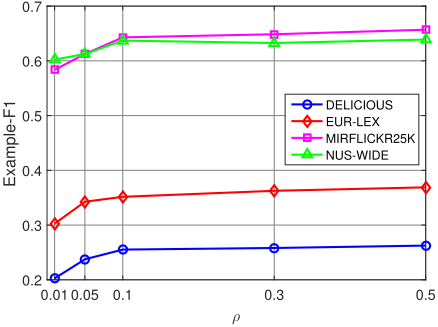
We study the sensitivity of the key parameter, i.e., ρ, in our proposed DBPC. ρ denotes the ratio between the sizes of prototype and database. The candidate set for ρ is [0.01, 0.05, 0.1, 0.3, 0.5]. The Example-F1 performance with respect to different ρ is shown in Figure 1. From this figure, we see that the accuracy improves as ρ increases from 0.01, and becomes steady after ρ reaches to around 0.1. The results reveal that a small subset of learned prototypes can represent the whole dataset well.
5 Conclusion
This work focuses on the challenging problem of speeding up kNN multi-label prediction. We propose a novel deep binary prototype compression (DBPC) that leverages a small set of binary codes to represent the whole database. Compared with advanced kNN embedding multi-label methods, DBPC enjoys both computational and memory efficiency. Extensive experiments on several large-scale datasets demonstrate that DBPC achieves several orders of magnitude lower storage and prediction complexity than state-of-the-art multilabel methods, while achieving very competitive accuracy.
Acknowledgments
This work was conducted within the Rolls-Royce@Nanyang Technological University Corporate Lab with support from the National Research Foundation (NRF) Singapore under the Corp Lab@University Scheme. Prof. Tsang is supported by ARC FT130100746, DP180100106 and LP150100671.
@inproceedings{ijcai2018p371,
  title     = {Deep Discrete Prototype Multilabel Learning},
  author    = {Shen, Xiaobo and Liu, Weiwei and Luo, Yong and Ong, Yew-Soon and Tsang, Ivor W.},
  booktitle = {Proceedings of the Twenty-Seventh International Joint Conference on
               Artificial Intelligence, {IJCAI-18}},
  publisher = {International Joint Conferences on Artificial Intelligence Organization},
  editor    = {Jérôme Lang},
  pages     = {2675--2681},
  year      = {2018},
  month     = {7},
  note      = {Main track},
  doi       = {10.24963/ijcai.2018/371},
  url       = {https://doi.org/10.24963/ijcai.2018/371},
}
TY - CPAPER TI - Deep Discrete Prototype Multilabel Learning AU - Shen, Xiaobo AU - Liu, Weiwei AU - Luo, Yong AU - Ong, Yew-Soon AU - Tsang, Ivor W. T2 - Proceedings of the Twenty-Seventh International Joint Conference on Artificial Intelligence, IJCAI-18 PB - International Joint Conferences on Artificial Intelligence Organization PY - 2018 SP - 2675 EP - 2681 DO - 10.24963/ijcai.2018/371 UR - https://doi.org/10.24963/ijcai.2018/371 ER -Copied
Machine-readable versions of this paper, for tools and AI agents:





