
A Bayesian Latent Variable Model of User Preferences with Item Context
Proceedings of the Twenty-Seventh International Joint Conference on Artificial Intelligence. Main track. Pages 2667-2674.
https://doi.org/10.24963/ijcai.2018/370
Keywords
- Machine Learning: Learning Generative Models
- Machine Learning: Recommender Systems
Abstract
Personalized recommendation has proven to be very promising in modeling the preference of users over items. However, most existing work in this context focuses primarily on modeling user-item interactions, which tend to be very sparse. We propose to further leverage the item-item relationships that may reflect various aspects of items that guide users' choices. Intuitively, items that occur within the same "context" (e.g., browsed in the same session, purchased in the same basket) are likely related in some latent aspect. Therefore, accounting for the item's context would complement the sparse user-item interactions by extending a user's preference to other items of similar aspects. To realize this intuition, we develop Collaborative Context Poisson Factorization (C2PF), a new Bayesian latent variable model that seamlessly integrates contextual relationships among items into a personalized recommendation approach. We further derive a scalable variational inference algorithm to fit C2PF to preference data. Empirical results on real-world datasets show evident performance improvements over strong factorization models.
- [Bishop, 2006] Christopher M Bishop. Pattern recognition and machine learning. springer, 2006.
- [Blei et al., 2017] David M Blei, Alp Kucukelbir, and Jon D McAuliffe. Variational inference: A review for statisti- cians. Journal of the American Statistical Association, 112(518):859-877, 2017.
- [Bobadilla et al., 2013] Jesús Bobadilla, Fernando Ortega, Antonio Hernando, and Abraham Gutiérrez. Recom- mender systems survey. Knowledge-based systems, 46:109-132, 2013.
- [Canny, 2004] John Canny. Gap: a factor model for discrete data. In Proceedings of the 27th International ACM SIGIR Conference, pages 122-129, 2004.
- [Cemgil, 2009] Ali Taylan Cemgil. Bayesian inference for nonnegative matrix factorisation models. Computational Intelligence and Neuroscience, 2009, 2009.
- [Chaney et al., 2015] Allison JB Chaney, David M Blei, and Tina Eliassi-Rad. A probabilistic model for using social networks in personalized item recommendation. In Pro- ceedings of ACM RecSys Conference, pages 43-50, 2015.
- [Charlin et al., 2015] Laurent Charlin, Rajesh Ranganath, James McInerney, and David M Blei. Dynamic poisson factorization. In Proceedings of the 9th ACM RecSys Con- ference, pages 155-162, 2015.
- [Friedman et al., 2001] Jerome Friedman, Trevor Hastie, and Robert Tibshirani. The elements of statistical learning, volume 1. Springer series in statistics New York, 2001.
- [Ghahramani and Beal, 2001] Zoubin Ghahramani and Matthew J Beal. Propagation algorithms for variational bayesian learning. In Advances in neural information processing systems, pages 507-513, 2001.
- [Gopalan et al., 2014a] Prem Gopalan, Francisco J Ruiz, Ra- jesh Ranganath, and David Blei. Bayesian nonparametric poisson factorization for recommendation systems. In Ar- tificial Intelligence and Statistics, pages 275-283, 2014.
- [Gopalan et al., 2014b] Prem K Gopalan, Laurent Charlin, and David Blei. Content-based recommendations with poisson factorization. In Advances in Neural Information Processing Systems, pages 3176-3184, 2014.
- [Gopalan et al., 2015] Prem Gopalan, Jake M Hofman, and David M Blei. Scalable recommendation with hierarchical poisson factorization. In UAI, pages 326-335, 2015.
- [Hu et al., 2008] Yifan Hu, Yehuda Koren, and Chris Volin- sky. Collaborative filtering for implicit feedback datasets. In IEEE ICDM, pages 263-272, 2008.
- [Jordan et al., 1999] Michael I Jordan, Zoubin Ghahramani, Tommi S Jaakkola, and Lawrence K Saul. An introduc- tion to variational methods for graphical models. Machine learning, 37(2):183-233, 1999.
- [Kingman, 1993] John Frank Charles Kingman. Poisson pro- cesses. Wiley Online Library, 1993. [Koenigstein et al., 2011] Noam Koenigstein, Gideon Dror, and Yehuda Koren. Yahoo! music recommendations: modeling music ratings with temporal dynamics and item taxonomy. In ACM RecSys, pages 165-172, 2011.
- [Koren et al., 2009] Yehuda Koren, Robert Bell, and Chris Volinsky. Matrix factorization techniques for recom- mender systems. Computer, 42(8), 2009.
- [Liang et al., 2016] Dawen Liang, Jaan Altosaar, Laurent Charlin, and David M Blei. Factorization meets the item embedding: Regularizing matrix factorization with item co-occurrence. In Proceedings of the 10th ACM RecSys Conference, pages 59-66, 2016.
- [Ma et al., 2008] Hao Ma, Haixuan Yang, Michael R Lyu, and Irwin King. Sorec: social recommendation using probabilistic matrix factorization. In Proceedings of the 17th ACM CIKM Conference, pages 931-940, 2008.
- [McAuley et al., 2015a] Julian McAuley, Rahul Pandey, and Jure Leskovec. Inferring networks of substitutable and complementary products. In Proceedings of the 21th ACM SIGKDD Conference, pages 785-794, 2015.
- [McAuley et al., 2015b] Julian McAuley, Christopher Tar- gett, Qinfeng Shi, and Anton Van Den Hengel. Image- based recommendations on styles and substitutes. In Pro- ceedings of the 38th International ACM SIGIR Confer- ence, pages 43-52, 2015.
- [Mnih and Salakhutdinov, 2008] Andriy Mnih and Ruslan R Salakhutdinov. Probabilistic matrix factorization. In Ad- vances in neural information processing systems, pages 1257-1264, 2008.
- [Park et al., 2017] Chanyoung Park, Donghyun Kim, Jinoh Oh, and Hwanjo Yu. Do also-viewed products help user rating prediction? In Proceedings of the 26th International Conference on World Wide Web, pages 1113-1122, 2017.
- [Rao et al., 2015] Nikhil Rao, Hsiang-Fu Yu, Pradeep K Ravikumar, and Inderjit S Dhillon. Collaborative filtering with graph information: Consistency and scalable meth- ods. In Advances in neural information processing sys- tems, pages 2107-2115, 2015.
- [Shan and Banerjee, 2010] Hanhuai Shan and Arindam Banerjee. Generalized probabilistic matrix factoriza- tions for collaborative filtering. In IEEE International Conference on Data Mining, pages 1025-1030, 2010.
- [Singh and Gordon, 2008] Ajit P Singh and Geoffrey J Gor- don. Relational learning via collective matrix factoriza- tion. In Proceedings of the 14th ACM SIGKDD Interna- tional Conference, pages 650-658, 2008.
- [Wang and Blei, 2011] Chong Wang and David M Blei. Col- laborative topic modeling for recommending scientific ar- ticles. In Proceedings of the 17th ACM SIGKDD Interna- tional Conference, pages 448-456, 2011.
- [Zhou et al., 2012] Tinghui Zhou, Hanhuai Shan, Arindam Banerjee, and Guillermo Sapiro. Kernelized probabilistic matrix factorization: Exploiting graphs and side informa- tion. In Proceedings of the SIAM International Conference on Data mining, pages 403-414, 2012.
References were extracted automatically from the PDF and may contain errors.
Full text extracted automatically from the PDF; figures, tables and equations may differ. The PDF is the version of record.
1 Introduction
Recommender systems are essential in guiding users as they navigate the myriads of options offered by modern applications. They rely chiefly on information about which items users have consumed-rated, purchased, etc.-in the past, which can be represented as user-item preference matrix. A predominant framework for recommendation is Matrix Factorization (MF) [Mnih and Salakhutdinov, 2008; Hu et al., 2008; Koren et al., 2009]. The principle is to decompose the preference matrix into low-dimensional user and item latent factor matrices. The bilinear combination of user and item's latent factors can be used to predict unknown preferences.
Classical probabilistic MF models [Mnih and Salakhutdinov, 2008] typically assume that a user's preference for an item is drawn from a Gaussian distribution centered at the inner product of their latent factor vectors. A distinct form of probabilistic MF, referred to as Poisson Factorization (PF) [Canny, 2004; Cemgil, 2009]-where the Poisson distribution is substituted for the usual Gaussian-recently demonstrates natural aptness for modeling discrete data such as ratings or purchases commonly found in recommendation scenarios. As documented in [Gopalan et al., 2015], thanks to the properties of the Poisson distribution, PF realistically models user preferences, fits well to sparse data, enjoys scalable variational inference with closed-form updates, and substantially outperforms previous state-of-the-art MF models based on Gaussian likelihoods [Mnih and Salakhutdinov, 2008; Shan and Banerjee, 2010; Koren et al., 2009].
Nevertheless, existing PF models for recommendation are primarily focused on user-item interactions, which are very sparse. A PF model that relies on user-item interactions alone may not necessarily associate similar items with similar representations in the latent space. This is due to the fact that such items are not necessarily rated by exactly the same users. Furthermore, on average, any given user may have had the opportunity to rate or purchase relatively few items. Thus, modeling and generalizing her preference across the large vocabulary of items based on the few user-item interactions alone is an onerous task. Fortunately, there are auxiliary information that could augment user-item interactions. One that we focus on in this paper is the contextual relationships among items.
Real-world behavior data often hold clues on how items may be related to one another. For instance, items found in the same shopping cart may work well together, e.g., shirt and matching pair of jeans. Items clicked or viewed on an e-commerce site in the same session may be alternatives for a particular need, e.g., shopping for a phone. Songs found in the same playlist probably share a coherent theme, e.g., country music of the 90s. As an abstraction of such scenarios, we introduce the notion of "context", which may refer to a shopping cart, session, playlist, etc., depending on the specific problem instance. Intuitively, items that share similar contexts are implicitly related to one another in terms of some aspect that guides the choices one makes, such as specification, functionality, visual appearance, compatibility, etc. Note that contextual relatedness is not necessarily synonymous with feature-based similarity, e.g., shirt and jeans may share similar contexts, though they have different features.
The question is how to exploit and incorporate such contextual relationships among items within the PF framework. In this work, we posit that there could be two reasons that might explain the preference of a user for an item. The first reason is that the user's latent preference matches the latent attributes of the item of interest. The second reason is that the user's latent preference matches those of other related items, i.e., those sharing similar contexts with the item of interest.
Based on the above assumption, we propose Collaborative Context Poisson Factorization (C2PF), a new Bayesian latent variable model of user preferences which takes into account contextual relationships between items; this is our first contribution. Under C2PF, the preference of a user for an item is driven by two components. One component is the interaction between the user's and item's latent factors, as in traditional PF. The other component consists of interactions between the user's latent factor and item's context latent factors. In this paper, "the context set of an item i" refers to the set of items sharing the same contexts (e.g., browsing sessions) with i. As the second contribution, we derive a scalable variational algorithm for approximate posterior inference, to fit our model to preference data. As the third contribution, through extensive experiments on six real-world datasets, we demonstrate the benefits of leveraging item context; C2PF noticeably improves upon the performance of Poisson factorization models, especially in the sparse scenario in which users express few ratings only.
2 RelatedWork
Given the breadth of scope of recommender systems in the literature [Bobadilla et al., 2013], we focus on those closely related to ours, to sharpen and clarify our contributions.
Approaches based on matrix factorization rely primarily on user-item interactions [Mnih and Salakhutdinov, 2008; Hu et al., 2008; Koren et al., 2009]. The sparsity of such information motivates the exploration of side information in several directions. On the users' side, these include leveraging social networks [Ma et al., 2008; Zhou et al., 2012] or common features [Rao et al., 2015] to bring related users' latent factors closer. On the items' side, these include exploiting item content [Wang and Blei, 2011] or product taxonomy [Koenigstein et al., 2011] to pull together item latent factors.
In this work, we focus on item-item relationships. The closest such work to ours is [Park et al., 2017], which proposes Matrix Co-Factorization (MCF) model. The latter falls into the large class of collective matrix factorization [Singh and Gordon, 2008], which consists in jointly decomposing multiple data matrices, user-item and item-item matrices in MCF, with shared latent factors. This is a widely used approach in the recommendation literature to exploit different sources of data. The model we propose is radically different from MCF. First, here we investigate another architecture for leveraging item relationships with new modeling perspectives. More precisely, as opposed to collective MF-based models like MCF, in our approach, the user-item preferences are the only observations being factorized, and the auxiliary information (item-item relationships) is embedded into the model's architecture. Second, MCF relies on the Gaussian distribution and uses stochastic gradient descent for learning, whereas our model builds on the Poisson distribution and enjoys scalable variational inference with closed-form updates. The benefits of our model are reflected in experiments.
In contrast, the CoFactor model [Liang et al., 2016] induces item relationships from the same user-item matrix, instead of a separate item-itemmatrix. It is also an instance of collective MF, relies on a Gaussian likelihood, and designed specifically for implicit feedback data [Hu et al., 2008].
Our model is also a novel contribution to the body of work on recommendation models based on Poisson factorization [Canny, 2004; Cemgil, 2009]. To our best knowledge, item context has not been explored within the PF framework.
Various other extensions of PF have been proposed. Gopalan et al. [2014a] develop Bayesian non-parametric PF, which does not require the dimension of the latent factors to be specified in advance. Gopalan et al. [2014b] propose Collaborative Topic Poisson Factorization (CTPF) to model both article contents and reader preferences. CTPF is also an instance of collective MF and could be viewed as a "Poisson" alternative to MCF. Chaney et al. [2015] extend PF to incorporate social interactions. Charlin et al. [2015] propose a model which accounts for user and item evolution over time.
3 Collaborative Context Poisson Factorization
This section describes Collaborative Context Poisson Factorization (C2PF), a Bayesian latent variable model of user preferences that accounts for the item's context.
Let X = (xui) denote the user-item preference matrix of size U ×I, where xui is the integer rating 1 that user u gave to item i, or zero if no preference was expressed. Let C = (cij ), of size I × J, be the item-context matrix, where cij = 1 if item j belongs to the context of item i, and cij = 0 otherwise. Subsequently, we refer to j as the context item, and to the set of items j for which cij = 1 as the context of item i.
C2PF builds on Poisson factorization [Friedman et al., 2001] to jointly model user preferences and leverage item's context. Formally, C2PF represents each user u with a vector of latent preferences θ⊤u ∈ RK+ , each item i with a vector of latent attributes β⊤i ∈ RK+ , and each context item j with a vector of latent attributes ξ⊤j ∈ RK+ . C2PF also assumes additional latent variables κij ∈ R+, one for each observed item-context pair, that we shall discuss shortly. Conditional on these latent variables, the user preferences xui are assumed to come from a Poisson distribution as follows:
The preference xui is affected by both how well the user u's latent factors θu matches the target item i's latent factors βi, and how well θu matches the context latent factors ξj of other items in i's context. Given that i may have multiple context items, it is natural to expect that different context items may affect i to different degrees. This is the intuition behind each variable κij, which represents the effect a context item j has on item i; we refer to these variables as the context effects.
The user latent preferences θuk, item attributes βik, context item attributes ξjk and context effects κij are all drawn from Gamma distributions. The Gamma is an exponential family distribution over positive random variables, governed by a shape and rate parameters [Bishop, 2006], which is a conjugate prior to the Poisson distribution.
1 Other user-item interactions indicative of preferences are also possible, e.g., number of clicks.
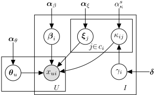
Moreover, in real-world data the items have very unbalanced context sizes, i.e., some have many more items in their context set than others. To account for this diversity in context size, C2PF assumes additional priors on the rate parameter of the Gamma distribution over the context effects κij, which govern the average magnitude of the latter variables. This induces a hierarchical structure over the κij's that makes it possible to model item context more realistically.
The graphical model of C2PF is depicted in Figure 1, and its generative process is as follows:
- Draw user preferences: θuk ∼ Gamma(αs θ , αrθ ).
- Draw context item attributes: ξjk ∼ Gamma(αs ξ , αr ξ ).
- For each item i:
- (a) Draw attributes: βik ∼ Gamma(αsβ , αrβ ).
- (b) Draw the average magnitude of the context effects: γi ∼ Inverse-Gamma(δs , δsc ).
- (c) For each context item j of i draw a context effect: κij ∼ Gamma(αsκ , αsκ γi ).
Note that C2PF includes as special cases other simpler models, such as the original Bayesian PF, which can be derived by modifying C2PF's specific components. In experiments, we consider some of such simpler variants of C2PF.
In practice, we are given X and C, and we are interested in reversing the above generative process so as to infer the posterior distribution of the latent user preferences, context effects, item and context item attributes, i.e., p(θ, β, ξ, κ|X, C). The latter will allow us to predict unknown ratings and generate recommendations. Once this posterior is fit, we can estimate the unknown ratings for each user-item pair (u, i) as follows:
where the expectation is with respect to the posterior. These predicted values are then used to rank unrated items for each user so as to provide him/her with a recommendation list.
As in many Bayesian models, exact posterior inference is challenging, i.e., the exact inference of the above posterior is intractable. We therefore resort to approximate inference.
4 Approximate Inference
Approximating the posterior is central to our work. In this section, we rely on variational inference and develop a scalable approximate inference algorithm for our model C2PF.
Variational Inference (VI) [Bishop, 2006] is a widely used approach in statistical learning to fit complex Bayesian models. This approach transforms the inference problem into an optimization problem. The key idea is to define a new posterior distribution q, governed by its own free variational parameters ν, that is tractable to work with. The objective is then to find the value of the variational parameters ν ∗ which indexes the distribution closest, in terms of the KullbackLeibler (KL) divergence, to the exact posterior. Finally, the resulting variational distribution q(.|ν ∗ ) is used as a surrogate to the true posterior in subsequent analysis.
We start by introducing an additional layer of auxiliary hidden variables, which leave the original model intact when marginalized out. For each observed rating xui we add K latent variables zx uik ∼ Poisson(θukβik) andK×ci. latent variables zcuijk ∼ Poisson(cijκijθukξjk), where ci. = ∑j cij. These auxiliary variables deterministically define the user preference. That is, xui = ∑k (zx uik + ∑j zcuijk ). The latter result follows from the additive property of Poisson random variables [Kingman, 1993], i.e., if x1 ∼ Poisson(λ1), x2 ∼ Poisson(λ2) and x = x1 + x2, then x ∼ Poisson(λ1 + λ2). Note that when xui is zero, zx uik and zcuijk are not random. This is why we consider these variables for the non-zero elements in X only. As we shall see, with these auxiliary variables in place our model is conditionally conjugate [Ghahramani and Beal, 2001], which will ease variational inference.
We now introduce our variational distribution q. We consider a mean-field family [Jordan et al., 1999], q(·|ν) = q(θ, β, ξ, κ, γ, Zx , Zc |ν), with a factorized form, i.e., the latent variables are assumed to be independent and each governed by its own variational parameters, as follows:
where ν = {λ, η, φ}. The form of each factor in the above equation is specified by the corresponding complete conditional: the conditional distribution of each variable given the other variables and observations. That is, the factors over the Gamma variables are also Gamma distributions with variational parameters λ, e.g., λθuk = (λθ,s uk , λθ,r uk ), the superscripts s and r refer to the shape and rate parameters.The factors over the Inverse-Gamma varibles γi are also Inverse-Gamma distribution with shape (s) and scale (sc) variational parameters, e.g., ηi = (ηs i , ηsc i ). Finally, the factors over zui = (zxui , zcui ) are Multinomial distributions with free parameters φui. The latter result follows from the fact that, the conditional distribution of a set of Poisson variables given their sum is a Multinomial; please refer to [Cemgil, 2009] for details.
Given the variational family q, VI is to fit its parameters by solving the following optimization problem:
This equation makes it clear how the observed data, X and C, enter the variational distribution. Once ν ∗ is found, we use q(·|ν ∗ ) as a surrogate to the true posterior to compute the prediction in (2) and subsequently make recommendations.
Coordinate ascent learning. We derive an efficient coordinate ascent mean-field algorithm to solve the optimization problem (4). The principle is to alternate the update of each variational parameter while holding the others fixed. Iterating on such updates is guaranteed to monotonically decrease the KL in (4), and to converge into a locally optimal solution.
Thanks to the auxiliary variables, our model is conditionally conjugate. That is, each complete conditional is in the exponential family [Ghahramani and Beal, 2001; Blei et al., 2017]. Thereby, each coordinate update can be performed in closed form, by setting the variational parameter equal to the expected natural parameter (w.r.t. q) of the corresponding complete conditional. This is indeed the optimal update for the variational parameter.
The complete conditional for the user preference, p(θuk|·), is a Gamma with shape and rate parameters given by:
The complete conditionals for the other Gamma variables are:
The complete conditional for the average intensity of the context effect is as follows:
The complete conditional for the auxiliary variables is:
where zui = (zxui , zcui ), pui = (pxui , pcui ) is a point on the (K +K × ci.)-simplex, and for all k, j: pxuik ∝ θukβik and pcuijk ∝ cijκijθukξjk.
The expected natural parameters (w.r.t. q) of these conditionals give the optimal updates for the variational parameters, e.g., the update for Gamma variational parameter λθuk is obtained by taking expectation of (5), which yields:
where we have used the standard results about the expectation of Gamma and Multinomial random variables. That is, if θ ∼ Gamma(λs , λr ), then E(θ) = λs λr , and if zui ∼ Multinomial(xui,φui), then the expectation of the kth component of zui is E(zuik) = xuiφuik. Using the standard results of the expectation of the log of a Gamma variable, i.e., E(log θ) = ψ(λs ) - log λr with ψ(·) denoting the digamma function, the updates for the components of the variational Multinomial parameter φui = (φxui , φcui ) are:
The updates for the remaining variational parameters can be derived in the same way. The full variational inference for C2PF is depicted in Algorithm 1.
Algorithm 1 Variational inference for C2PF.
Input: X, C, K, δ , αθ, αβ, αξ, αsκ
Output: The set of variational parameters ν ∗
Steps:
1. Initialization: ηs i = δs + ci. × αsκ, randomly initialize the remaining Gamma variational parameters λs , λr
repeat
2. For each observed preference xui, update the variational Multinomial parameter φui using equations (12) and (13).
3. Update the user related parameters, ∀u, k:
until convergence
Efficient implementation. A key property of the variational C2PF algorithm is efficiency. The operations involving users and items need to be carried out for only the non-zero elements in X and C. Furthermore, we can avoid explicitly computing and storing the Multinomial parameters φ. We need to store only the following matrices, Lθ = (exp{Eq(log θuk)}), Lβ = (exp{Eq(logβik)}), Lξ = (exp{Eq(log ξjk)}) and Lκ = (exp{Eq(logκij)}). We can then use these quantities directly in the updates of the variational shape parameters.
Computational time complexity. The Proposition below shows that the computational complexity of Algorithm 1 scales linearly with the number of non-zero entries in X and C. In practice X and C are extremely sparse, and Algorithm 1 converges within 100 iterations. Furthermore, the updates of the variational parameters are trivially parallelizable across users and items, hence our variational inference for C2PF can easily scale to large datasets.
Proposition 1. Let nzx and nzc denote respectively the number of non-zero in X and C. The computational complexity per iteration of Algorithm 1 is O(K · (nzx + nzc + U + I)).
Proof. The computation bottleneck of Algorithm 1 is with the update blocks 3 to 6. The computational complexity of updating λθ,s uk is O(nzu x ), such that nzu x is the number of ratings expressed by user u. This complexity holds since the sum over j can be precomputed once for each i,k and stored in a I × K matrix, the total cost of this operation is O(K · nzc). The complexity of updating all λθ,r uk parameters is O(K · (I +U + nzc)). Therefore, the computational complexity of block 3 is O(K · (nzx + nzc + U + I)).
Similarly, we can show that the complexity of block 4 is O(K · (nzx + U + I)) and that of blocks 5 and 6 is O(K · (nzc +nzx +U +J)). Putting it all together, the complexity per iteration of Algorithm 1 is O(K · (nzx + nzc + U + I)), where we have assumed that I is of the same order as J.■
5 Experimental Study
Our objective is to study the impact of item context, and our modeling assumptions, on personalized recommendation.
5.1 Datasets
We use six datasets from Amazon.com 2 , provided by McAuley et al.; McAuley et al. [2015b; 2015a]. These datasets include both the user-item preferences and the "Also Viewed" lists that we treat as the item contexts. We preprocess all datasets so that each user (resp. item) has at least ten (resp. two) ratings, and the sets of items and context items are identical. Table 1 describes the resulting datasets.
| Datasets | Characteristics | |||||
|---|---|---|---|---|---|---|
| #Users | #Items | #Ratings | nzX (%) | #nzC | nzC (%) | |
| Office | 3,703 | 6,523 | 53,282 | 0.22 | 108,466 | 0.25 |
| Grocery | 8,938 | 22,890 | 148,735 | 0.07 | 480,300 | 0.09 |
| Automotive | 7,280 | 15,635 | 63,477 | 0.05 | 365,634 | 0.15 |
| Sports | 19,049 | 24,095 | 211,582 | 0.04 | 531,148 | 0.09 |
| Pet Supplies | 16,462 | 20,049 | 164,017 | 0.05 | 631,102 | 0.16 |
| Clothing | 41,809 | 97,619 | 420,377 | 0.01 | 1,080,442 | 0.01 |
5.2 Comparative Models
We benchmark our model, C2PF, against strong comparable generative factorization models.
- MCF: Matrix Co-Factorization [Park et al., 2017], which incorporates item-to-item relationships into Gaussian MF.
- PF: Bayesian Poisson Factorization [Gopalan et al., 2015] which arises as a special case from our model without the item context. Therefore, we can effectively assess the impact of the item context by comparing C2PF to PF.
- CTPF: Collaborative Topic Poisson Factorization [Gopalan et al., 2014b] is a co-factorization approach that jointly models user preferences and item topics. It can also be used to leverage the item context by substituting the itemcontext matrix C for the item-word matrix.
- CoCTPF: Content-only CTPF [Gopalan et al., 2014b] is a variant of CTPF without the document topic offsets; please refer to [Gopalan et al., 2014b] for details.
2 http://jmcauley.ucsd.edu/data/amazon/
Note that the above baselines have been found to perform better than several other models on the task of item recommendation. To examine the contributions of our modeling choices, we also include the results for two simplified variants of C2PF.
- rC2PF: reduced C2PF that drops the item factors β, resulting in a simpler model where only the context part in (1) is responsible for explaining the user preferences xui 3 ,
- tC2PF: tied C2PF that constrains the context factors ξ to be the same as the item factors β, that is ξi = βi for all i.
5.3 Experimental Settings
For each dataset, we randomly select 80% of the ratings as training data and the remaining 20% as test data. Random selection is carried out five times independently on each dataset. The average performance over the five samples is reported as the final result.
For most experiments, we set the number of latent components K to 100. Later, we will also vary K and indeed find 100 to be a good trade-off between accuracy and model complexity. To encourage sparse latent representations, we set αθ = αβ = αξ = (0.3, 0.3) -resulting in exponentially shaped Gamma distributions with mean equal to 1. We further set δ = (2, 5) and αsκ = 2, fixing the prior mean over the context effects to 0.5. Note that we set αsκ > 1 to avoid sparse distributions over the κij variables and thereby encourage C2PF to rely on item's context to explain user preferences. For an illustration, please refer to Figure 2 in [Cemgil, 2009]. We initialize the Gamma variational parameters, λs and λr , to a small random perturbation of the corresponding prior parameters. In order for the comparisons to be fair, we use the same initial parameters for all PF-based models, where it is possible.
To set the different hyperparameters of MCF, we follow the same strategy, grid search, as in [Park et al., 2017].
5.4 EvaluationMetrics
We assess the recommendation accuracy on a set of held-out items-the test set. We retain four widely used measures for top-M recommendation, namely the Normalized Discount Cumulative Gain (nDCG), Mean Reciprocal Rank (MRR), Precision@M (P@M) and Recall@M (R@M), where M is the number of items in the recommendation list [Bobadilla et al., 2013]. Intuitively, nDCG and MRR measures the raking quality of a model, while Precision@M and Recall@M assess the quality of a user's top-M recommendation list. These measures vary from 0.0 to 1.0 (higher is better).
5.5 Empirical Results and Discussion.
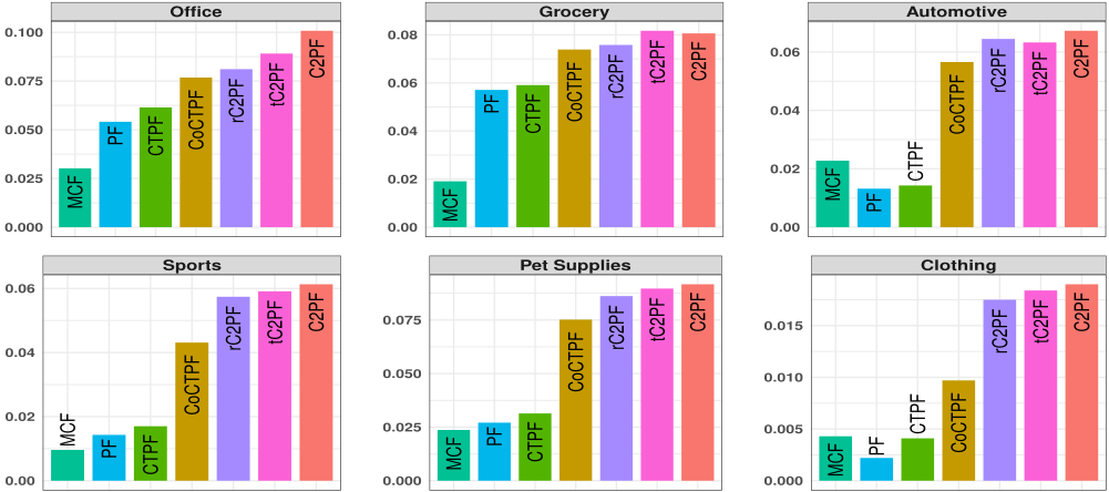
Table 2 depicts the average performances of the various competing models in terms of different metrics, over all datasets. In order to ease interpretation, we provide another presentation of Recall@20 in Figure 2-the results are consistent across all metrics.
We note that C2PF, and its variants, substantially outperforms the other competing models on all datasets and across all measures. Recall that without the item context information C2PF degenerates to the basic PF. We can therefore attribute the performance improvements reached by C2PF, relative to PF, to the modeling of the item context. The importance of the item context is also strongly supported by the high performance of rC2PF relative to PF, though rC2PF relies solely on item's context to make recommendations.
3 This variant considers only items with non-empty context sets since the rate of the Poisson cannot be zero
| Data | Metric | MCF | PF | CTPF | CoCTPF | rC2 PF | tC2 PF | C2 PF |
|---|---|---|---|---|---|---|---|---|
| Office Prod | nDCG | 0.1525 | 0.1663 | 0.1718 | 0.1806 | 0.1870 | 0.1921 | 0.2005 |
| MRR | 0.0239 | 0.0414 | 0.0467 | 0.0558 | 0.0596 | 0.0674 | 0.0770 | |
| P@10 | 0.0052 | 0.0107 | 0.0123 | 0.0148 | 0.0156 | 0.0174 | 0.0197 | |
| R@10 | 0.0195 | 0.0290 | 0.0344 | 0.0446 | 0.0512 | 0.0566 | 0.0637 | |
| P@20 | 0.0041 | 0.0096 | 0.0111 | 0.0129 | 0.0133 | 0.0143 | 0.0160 | |
| R@20 | 0.0302 | 0.0541 | 0.0615 | 0.0768 | 0.0811 | 0.0891 | 0.1008 | |
| Grocery | nDCG | 0.1286 | 0.1568 | 0.1553 | 0.1717 | 0.1722 | 0.1776 | 0.1763 |
| MRR | 0.0145 | 0.0452 | 0.0429 | 0.0529 | 0.0590 | 0.0595 | 0.0585 | |
| P@10 | 0.0031 | 0.0115 | 0.0118 | 0.0136 | 0.0145 | 0.0157 | 0.0151 | |
| R@10 | 0.0122 | 0.0343 | 0.0358 | 0.0440 | 0.0478 | 0.0519 | 0.0500 | |
| P@20 | 0.0024 | 0.0095 | 0.0095 | 0.0116 | 0.0114 | 0.0128 | 0.0121 | |
| R@20 | 0.0191 | 0.0571 | 0.0591 | 0.0739 | 0.0758 | 0.0817 | 0.0806 | |
| Automotive | nDCG | 0.1186 | 0.1123 | 0.1124 | 0.1417 | 0.1462 | 0.1460 | 0.1468 |
| MRR | 0.0121 | 0.0100 | 0.0103 | 0.0337 | 0.0394 | 0.0387 | 0.0392 | |
| P@10 | 0.0028 | 0.0019 | 0.0021 | 0.0075 | 0.0087 | 0.0087 | 0.0093 | |
| R@10 | 0.0151 | 0.0088 | 0.0094 | 0.0351 | 0.0417 | 0.0415 | 0.0439 | |
| P@20 | 0.0022 | 0.0015 | 0.0016 | 0.0058 | 0.0069 | 0.0066 | 0.0070 | |
| R@20 | 0.0228 | 0.0132 | 0.0143 | 0.0566 | 0.0645 | 0.0633 | 0.0673 | |
| Sports | nDCG | 0.1122 | 0.1179 | 0.1189 | 0.1398 | 0.1512 | 0.1521 | 0.1547 |
| MRR | 0.0071 | 0.0122 | 0.0119 | 0.0297 | 0.0390 | 0.0409 | 0.0427 | |
| P@10 | 0.0015 | 0.0022 | 0.0026 | 0.0067 | 0.0091 | 0.0093 | 0.0096 | |
| R@10 | 0.0061 | 0.0083 | 0.0101 | 0.0266 | 0.0361 | 0.0374 | 0.0393 | |
| P@20 | 0.0011 | 0.0018 | 0.0022 | 0.0054 | 0.0072 | 0.0073 | 0.0076 | |
| R@20 | 0.0096 | 0.0143 | 0.0170 | 0.0431 | 0.0574 | 0.0591 | 0.0613 | |
| Pet Supplies | nDCG | 0.1201 | 0.1288 | 0.1317 | 0.1585 | 0.1627 | 0.1628 | 0.1678 |
| MRR | 0.0136 | 0.0207 | 0.0237 | 0.0441 | 0.0501 | 0.0516 | 0.0562 | |
| P@10 | 0.0028 | 0.0039 | 0.0048 | 0.0103 | 0.0110 | 0.0113 | 0.0122 | |
| R@10 | 0.0147 | 0.0184 | 0.0219 | 0.0499 | 0.0526 | 0.0550 | 0.0597 | |
| P@20 | 0.0022 | 0.0029 | 0.0034 | 0.0079 | 0.0089 | 0.0091 | 0.0095 | |
| R@20 | 0.0237 | 0.0271 | 0.0314 | 0.0752 | 0.0862 | 0.0897 | 0.0917 | |
| Clothing | nDCG | 0.0896 | 0.0885 | 0.0896 | 0.0961 | 0.1014 | 0.1046 | 0.1061 |
| MRR | 0.0031 | 0.0018 | 0.0032 | 0.0065 | 0.0118 | 0.0122 | 0.0130 | |
| P@10 | 0.0006 | 0.0003 | 0.0006 | 0.0013 | 0.0020 | 0.0023 | 0.0026 | |
| R@10 | 0.0028 | 0.0014 | 0.0028 | 0.0062 | 0.0111 | 0.0114 | 0.0120 | |
| P@20 | 0.0004 | 0.0002 | 0.0005 | 0.0010 | 0.0016 | 0.0019 | 0.0021 | |
| R@20 | 0.0043 | 0.0022 | 0.0041 | 0.0097 | 0.0175 | 0.0184 | 0.0190 |
Overall, the results from Table 2 suggest that the item context underlies different aspects of items that explain the user behaviour. To gain further insights into the performance of the proposed model and the impact of our modeling choices, we now delve into specific research questions.
- Q1. How important is the Poisson distribution? We observe that even though PF does not leverage the relationships among items, it still outperforms MCF in most cases. This provides empirical evidence that the Poisson distribution is a better alternative to Gaussian in modeling user preferences.
- Q2. How important are the C2PF's modeling assumptions? CTPF and CoCTPF offer alternative PF-based architectures to C2PF for leveraging item's context, with different modeling assumptions. More precisely, CTPF and CoCTPF fall into the class of collective matrix factorization, and consist in jointly factorizing the user-itemX and item-context C matrices, with shared item factors. This is a popular strategy in the recommendation literature to model different sources of data. The proposed models, C2PF and its variants, substantially outperform CTPF and CoCTPF in all cases, demonstrating the benefits of the assumptions behind C2PF.
- Q3. Why does CoCTPF performs better than CTPF? CoCTPF arises as a special case from CTPF without the item offset. Surprisingly, the former performs better than the latter. A careful investigation reveals that the magnitudes of the item offsets (noted ϵ in the original paper) tend to be bigger than those of the shared item attributes θ. This means that, in CTPF, the item offsets, which are specific to
contribute to explain user behaviour, but so do their contexts. Empirical results on real-world datasets show that C2PF noticeably improves the performance of Poisson factorization models, especially in the sparse scenario in which users express few ratings, suggesting that the item context underlies aspects of items that can explain the user preferences.
A flexible model with strong theoretical foundations, C2PF can be extended in several directions. For instance, it would be interesting to extend C2PF to account for user-user social relationships to further alleviate the sparsity issue. Another possible line of future work is to compose C2PF with other graphical models. For instance, one could combine C2PF and CTPF to jointly model item's context and textual content.
Acknowledgments
This research is supported by the National Research Foundation, Prime Minister's Office, Singapore under its NRF Fellowship Programme (Award No. NRF-NRFF2016-07).
the user-item interaction component, dominate the prediction of unknown preferences (please refer to equation 1 in [Gopalan et al., 2014b]).
- Q4. When does C2PF offer the most improvements?
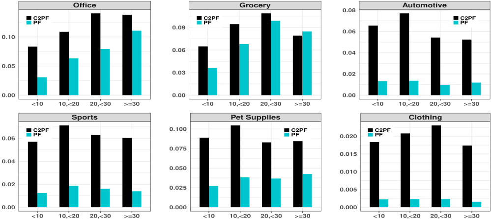
- In Figure 3, we report the performances, in terms of Recall@20, of C2PF and PF, on users with different number of ratings. C2PF consistently achieves the best performance over different scenarios. Though this may be datadependent, C2PF seems to provide the most improvement on users with few ratings. The relative difference between C2PF and PF tends to decrease with more ratings. It is challenging to infer good user representations when there is a lack of information in the preference matrix. By leveraging additional signals from items' contexts, C2PF mitigates this lack of information.
- Q5. What is the impact of the number of factors on the performance of C2PF?
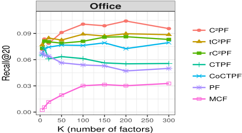
In Figure 4, we report the performance of the different models, on Office, over different K. C2PF consistently outperforms the competing methods. It is not very sensitive to the value of K and seems to provide better performances when K ≥ 100. Because the complexity of the models increases with K, we recommend to set the number of factors to 100, which is a good tradeoff between recommendation quality and model complexity.
6 Conclusion &Perspectives
Based on the assumption that items sharing similar contexts are related in some latent aspect that guides one's choices, we develop Collaborative Context Poisson Factorization (C2PF), a Bayesian latent factor model of user preferences which takes into account the contextual relationships among items. Under C2PF, not only do items (through latent attributes)
@inproceedings{ijcai2018p370,
  title     = {A Bayesian Latent Variable Model of User Preferences with Item Context},
  author    = {Salah, Aghiles and Lauw, Hady W.},
  booktitle = {Proceedings of the Twenty-Seventh International Joint Conference on
               Artificial Intelligence, {IJCAI-18}},
  publisher = {International Joint Conferences on Artificial Intelligence Organization},
  editor    = {Jérôme Lang},
  pages     = {2667--2674},
  year      = {2018},
  month     = {7},
  note      = {Main track},
  doi       = {10.24963/ijcai.2018/370},
  url       = {https://doi.org/10.24963/ijcai.2018/370},
}
TY - CPAPER TI - A Bayesian Latent Variable Model of User Preferences with Item Context AU - Salah, Aghiles AU - Lauw, Hady W. T2 - Proceedings of the Twenty-Seventh International Joint Conference on Artificial Intelligence, IJCAI-18 PB - International Joint Conferences on Artificial Intelligence Organization PY - 2018 SP - 2667 EP - 2674 DO - 10.24963/ijcai.2018/370 UR - https://doi.org/10.24963/ijcai.2018/370 ER -Copied
Machine-readable versions of this paper, for tools and AI agents:





