
An Information Theory based Approach to Multisource Clustering
Proceedings of the Twenty-Seventh International Joint Conference on Artificial Intelligence. Main track. Pages 2581-2587.
https://doi.org/10.24963/ijcai.2018/358
Keywords
- Machine Learning: Multi-instance;Multi-label;Multi-view learning
- Machine Learning: Clustering
Abstract
Clustering is a compression task which consists in grouping similar objects into clusters.
In real-life applications, the system may have access to several views of the same data and each view may be processed by a specific clustering algorithm: this framework is called multi-view clustering and can benefit from algorithms capable of exchanging information between the different views.
In this paper, we consider this type of unsupervised ensemble learning as a compression problem and develop a theoretical framework based on algorithmic theory of information suitable for multi-view clustering and collaborative clustering applications.
Using this approach, we propose a new algorithm based on solid theoretical basis, and test it on several real and artificial data sets.
- [Bickel and Scheffer, 2005] Steffen Bickel and Tobias Scheffer. Estimation of mixture models using co-em. In João Gama, Rui Camacho, Pavel Brazdil, Alípio Jorge, and Luís Torgo, editors, Machine Learning: ECML 2005, 16th European Conference on Machine Learning, Porto, Portugal, October 3-7, 2005, Proceedings, volume 3720 of Lecture Notes in Computer Science, pages 35-46. Springer, 2005.
- [Cleuziou et al., 2009] Guillaume Cleuziou, Matthieu Exbrayat, Lionel Martin, and Jacques-Henri Sublemon- tier. Cofkm: A centralized method for multiple-view clustering. In Wei Wang, Hillol Kargupta, Sanjay Ranka, Philip S. Yu, and Xindong Wu, editors, ICDM 2009, The Ninth IEEE International Conference on Data Min- ing, Miami, Florida, USA, 6-9 December 2009, pages 752-757. IEEE Computer Society, 2009.
- [Cornuéjols et al., 2018] Antoine Cornuéjols, Cédric Wem- mert, Pierre Ganc ¸arski, and Younès Bennani. Collabora- tive clustering: Why, when, what and how. Information Fusion, 39:81-95, 2018.
- [D.L. Davies, 1979] D.W. Bouldin D.L. Davies. A cluster separation measure. IEEE Trans. Pattern Anal. Machine Intell., 1 (4):224-227, 1979.
- [Filali et al., 2016] A. Filali, C. Jlassi, and N. Arous. Som variants for topological horizontal collaboration. In 2016 2nd International Conference on Advanced Technologies for Signal and Image Processing (ATSIP), pages 459-464, March 2016.
- [Forestier et al., 2007] G. Forestier, C. Wemmert, and P. Gancarski. Collaborative multi-strategical classification for object-oriented image analysis. In Workshop on Super- vised and Unsupervised Ensemble Methods and Their Ap- plications in conjunction with IbPRIA, pages 80-90, June 2007.
- [Ghassany et al., 2012] Mohamad Ghassany, Nistor Grozavu, and Younès Bennani. Collaborative clus- tering using prototype-based techniques. International Journal of Computational Intelligence and Applications, 11(3), 2012.
- [Grozavu and Bennani, 2010] Nistor Grozavu and Younès Bennani. Topological collaborative clustering. Australian Journal of Intelligent Information Processing Systems, 12(3), 2010.
- [Hutter, 2000] M. Hutter. A theory of universal artificial in- telligence based on algorithmic complexity. Technical re- port, April 2000.
- [Li and Vitanyi, 2008] Ming Li and Paul M.B. Vitanyi. An Introduction to Kolmogorov Complexity and Its Applica- tions. Springer Publishing Company, Incorporated, 3 edi- tion, 2008.
- [Nistor Grozavu, 2009] Younès Bennani Mustapha Lebbah Nistor Grozavu. From variable weighting to cluster char- acterization in topographic unsupervised learning. In in Proc. Proc. of IJCNN09, International Joint Conference on Neural Network, 2009.
- [Pedrycz, 2002] Witold Pedrycz. Collaborative fuzzy clus- tering. Pattern Recognition Letters, 23(14):1675-1686, 2002.
- [Rand, 1971] W.M. Rand. Objective criteria for the evalua- tion of clustering methods. Journal of the American Sta- tistical Association., pages 846-850, 1971.
- [Rissanen, 1978] J. Rissanen. Modeling by shortest data de- scription. Automatica, 14(5):465 -471, 1978.
- [Rougier and Puissant, 2014] S. Rougier and A. Puissant. Improvements of urban vegetation segmentation and clas- sification using multi-temporal pleiades images. 5th Inter- national Conference on Geographic Object-Based Image Analysis, page 6, 2014.
- [Rousseeuw, 1987] R.J. Rousseeuw. Silhouettes: a graphical aid to the interpretation and validation of cluster analy- sis. Journal of Computational and Applied Mathematics., 20:53-65, 1987.
- [Solomonoff, 1964] Ray J Solomonoff. A formal theory of inductive inference. part i. Information and control, 7(1):1-22, 1964.
- [Sublime et al., 2017] Jérémie Sublime, Basarab Matei, Guénael Cabanes, Nistor Grozavu, Younès Bennani, and Antoine Cornuéjols. Entropy Based Probabilistic Collabo- rative Clustering. Pattern Recognition, 72:144-157, 2017.
- [Vanhaesebrouck et al., 2017] Paul Vanhaesebrouck, Aurélien Bellet, and Marc Tommasi. Decentralized Collaborative Learning of Personalized Models over Networks. In AISTATS, 2017.
- [Wallace and Boulton, 1968] C. S. Wallace and D. M. Boul- ton. An information measure for classification. The Com- puter Journal, 11(2):185-194, 1968.
- [Wemmert and Gancarski, 2002] Cedric Wemmert and Pierre Gancarski. A multi-view voting method to combine unsupervised classifications. Artificial Intelligence and Applications, Malaga, Spain,, pages 447 -452, 2002.
- [Zimek and Vreeken, 2015] Arthur Zimek and Jilles Vreeken. The blind men and the elephant: on meeting the problem of multiple truths in data from clustering and pattern mining perspectives. Machine Learning, 98(1-2):121-155, 2015.
References were extracted automatically from the PDF and may contain errors.
Full text extracted automatically from the PDF; figures, tables and equations may differ. The PDF is the version of record.
1 Introduction
Multi-source data is a never ending source of information that is produced daily and must be processed by Machine Learning algorithms. They come from the Internet where data is available from multiple sources for the same users (such as social networks), but it can also be found in medical diagnosis where multiple tests are run for the same patients, and finally teledetection also produces a lot of complex multi-view data where multiple types of color and texture attributes can be used to describe larges images. The unsupervised exploration and analysis of such data sets is a complex process which gave birth to several recent fields of research in Machine Learning. Multi-view clustering [Zimek and Vreeken, 2015] and collaborative clustering methods [Cornu´ejols et al., 2018; Vanhaesebrouck et al., 2017] are the two main families of algorithms to process such data. Both types of methods use several clustering algorithms to mine information locally in each view and then share these information between the different algorithms. From there, the main difference between the two is that collaborative clustering only aims at sharing the information between the local algorithms with a goal of mutual improvement, while multi-view clustering shares the information and then aims at finding a single consensus clustering partition. The two families of methods therefore share closely related issues and feature similar algorithms. The main weakness of the methods proposed in both fields is that, in most methods, the multi-view clustering or collaboration can work only between very similar clustering algorithms, thus reducing the diversity of methods that can be used. The literature features solutions where C-Means algorithms can collaborate together [Pedrycz, 2002], GMM can work together [Bickel and Scheffer, 2005; Cleuziou et al., 2009], SOM or GTM can collaborate together [Ghassany et al., 2012; Filali et al., 2016], etc.
Within this context, in this paper we propose a new setting for collaborative clustering (without consensus global solution), the aim of which is to be generic enough to enable any type of clustering algorithm to work together within the same collaborative or multi-view context. To do so, we use a collaborative fitness function based on Kolmogorov complexity that can be used on any type of clustering local model to efficiently evaluate and reduce the distance between clustering partitions.
This proposed collaborative algorithm can be seen as an improvement on a previous collaborative framework that already encompassed any probabilistic clustering method [Sublime et al., 2017]. In our case, we are not limited to probabilistic clustering so long as the Kolmogorov complexity of the local model can be computed. Furthermore, our model gives a better justification for the general form of the collaborative term. Another similar method is the SAMARA method [Wemmert and Gancarski, 2002; Forestier et al., 2007] which was designed to merge solutions from different clustering algorithms applied to image processing. The main limits of this latter approach are that 1) it discards completely the local term which makes the specificity of the local algorithms, 2) the merging method is based on a conflict resolution algorithm somewhat similar to what we propose, but based on an arbitrary criterion with little theoretical justification. By contrast, our method uses a solid theoretical basis on information theory with Kolmogorov complexity.
The remainder of this article is organized as follows: In Section 2, we present the general idea of the method and define a restricted universal Turing machine adapted to multisource clustering. In Section 3, we expose an algorithmbased on the presented framework. Applications of this algorithm on artificial and real data sets is presented in Section 4. We eventually discuss the advantages of our method and its potential improvements in Section 5.
2 Collaboration withMinimumDescription Length principle
2.1 Reminder: Kolmogorov Complexity
A long philosophical tradition has investigated the problem of induction. Among the proposed methodologies, Ockham's razor is widely used and discussed. This simplicity principle states that, among all possible hypotheses, only the "simplest" one should be chosen to describe an observation. A more formal version of this idea has been introduced in computer science by [Wallace and Boulton, 1968] and [Rissanen, 1978] with the Minimum Description Length (MDL) principle. This principle states that the best model to select leads to a maximal compression of observed data.
The notion of description length originates from algorithmic theory of information and designates the minimal number of bits needed by a Turing machine to describe an object [Li and Vitanyi, 2008]. This measure is given by the tool of Kolmogorov complexity. If M is a fixed Turing machine, the complexity of an object x given an object y on machine M is defined as KM(x|y) = minp∈PM {l(p) : p(y) = x} where PM is the set of programs onM, p(y) designates the output of program p with argument y and l measures the length (in bits) of a program. When the argument y is empty, we use the notation KM(x) and call this quantity the complexity of x.
2.2 Fixing the Machine
With this definition, the complexity of an object cannot be considered as an intrinsic property of the object since it depends on a fixed Turing machine M. In order to overcome this weakness, the invariance theorem enables to define a machine-independent definition of the complexity. Although such a measure has a major theoretical impact (see for instance [Solomonoff, 1964; Hutter, 2000]), we will focus on a machine-dependent approach in the rest of this paper. Our choice is motivated by three main reasons exposed thereafter.
First, the universal complexity is not computable, since it is defined as a minimum over all programs of all machines. By choosing a precise machine, we restrict the research to a minimization over the set of programs only, which can be relatively simple depending on the chosen machine.
Secondly, machine dependency is a fundamental property of learning. It is intuitively obvious that all learners have their own data processing, and thus are naturally biased toward some precise tasks. For instance, human mind is designed to perceive some regularities in scenes that state-of-the-art algorithms cannot get, while they are unable to cope with pattern recognition in strings like DNA, which is now a basic task for a computer program. Since any learning method has a natural bias toward some kinds of problems, we propose here to interpret this property in terms of machine dependency: A learning algorithm corresponds to a specific choice of a Turing machine with its representation bias.
Finally, we have to notice that this assumption is a classical assumption in statistical learning theory. The restriction of the research space to classes of decision functions (hence classes of Turing machines) is even the key hypothesis in learning theory and leads to all classical definitions such as the VC-dimension in supervised learning. Statistical learning relies on this very assumption: because of the noncalculability of probabilities and in order to prevent overfitting (i.e. to reject distributions which do not obey the commonly admitted aim of generalization), the assumption of choosing a restricted set of hypotheses is well accepted in the machine learning field.
In the following, we consider that the machine M is fixed. To make the equations easier to read, we will omit to specify the machine M in the complexity (hence we will denote by K(x) the complexity of x on the chosen machine). The purpose of the following section is to describe a class of Turing machines which is adapted to the multi-view setting.
2.3 Local Sub-Machine
Given multi-view data, the purpose here is to define a parameterized class of Turing machines M which generate the data. In a multi-source setting, and without any loss of generality, we consider that each view is encoded on a tape. We consider that data points are encoded in a given (and known) order and are separated, in such a way that the content of a tape can be uniquely decoded.
Local clustering (ie. clustering on a single view) can be interpreted as a compression of data based on external parameters. For instance, a centroid-based clustering (like K-means, K-medoids or GTM) compresses the data by "factorizing" a common position into the center. We propose to define local sub-machines as machines which take as input a parameter θj and a solution vector Sj and output the corresponding data. The length of such machines is equal to K(Xj |Sj , θj ).
The format of these machines will depend on the nature of the clustering algorithms. It is noticeable that the framework of algorithmic learning theory authorizes a large class of data representations (and thus can be used for collaboration between different types of clustering methods). We provide a couple of examples in the following:
- Prototype-based models (K-means, K-medoids, GTM, SOM...): the parameter θj is the description of the prototypes. Each data point is represented by its membership to its associated prototype (the association table being given by the solution vector Sj )
- Probabilistic models (GMM...): the parameter θj describe the probability distribution inferred by the system. In general, this distribution is parametric and θj can be associated to the parameters of the distribution. The description length of data X knowing a distribution µ is given by the relation K(X|µ) = - log µ(X).
- Density-based models (DBSCAN, OPTICS...): Even if such models do not rely on a direct descriptive model, it is possible to consider θ as a data reordering. The
total data set description is then based on the position of previous points in the new order.
2.4 FromGlobal Parameters to Local Views
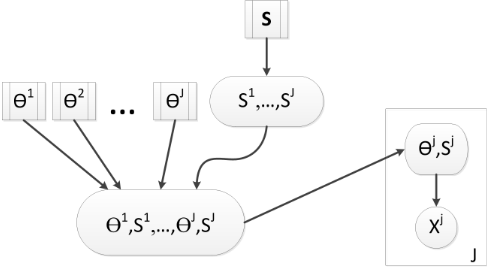
We propose a decomposition of the global Turing machine into sub-machines, as exposed in Figure 1. In order to make the description more understandable, we invite the reader to think of machines as actual computer programs and the complexity (also called length) as the length of the program as written in a fixed programming language.
The j-th local sub-machine is in charge of producing data Xj from the clustering parameter θj and the solution vector Sj , received as inputs. These parameters were transferred to it from a global configuration machine which stores the whole configuration (ie. the complete description of all θj s and Sj s). A splitting operation is needed to transform the output 〈θ1 , S1 , . . . , θJ , SJ 〉 of the global configuration machine into the inputs 〈θj , Sj 〉 of the local sub-machines. Since we use prefix codes and the index j of the parameters θj and Sj is explicitly given onto the tape of the global sub-machine, the complexity of this splitting operation is a constant which does not depend on the data nor on the parameters.
The global configuration machine receives as input the local parameters θ1 , . . . , θJ and a global solution vector 〈S1 , . . . , S J 〉. The length of this machine corresponds to the description length of the parameters θ and the cost of a concatenation (hence a constant). The complexity of the local solutions is measured by the description length of the sub-machine in charge of their generation.
The key of collaboration lies in the construction of the local solutions 〈S1 , . . . , S J 〉. This construction relies on a global unknown solution S which might be interpreted as a consensus. The nature of parameter S will be discussed later: In this section, we only consider it as a global parameter used for the construction of local solutions. For each view j, a sub-machine computes Sj from the global solution S. The length of this sub-machine is ∑Jj=1 K(Sj |S). Designing the index j counts as a constant in the complexity and thus is not indicated.
2.5 Complexity of aMachine
The architecture of the described machine is summed up in Figure 1. The machines described by such a schema constitute a parametric machine class given with parameters θ1 , S1 , . . . , θJ , SJ , S. The length of a machine in this class, up to an additive constant, is given by:
Minimum Description Length principle states that the model chosen to describe data is associated to the machine of minimal length. As a consequence, the problem of interest for multi-source clustering in the proposed framework is the following: minimize
where l is given in Equation 1 and Mθ1 ,S1 ,...,θJ ,SJ ,S designates the Turing machine in the restricted class with indicated parameters.
This minimization problem presents interesting properties: the first one is the genericity of the formula in Equation 1 which has the exact same form as state of the art methods for multi-source clustering [Cornu´ejols et al., 2018]. It can be divided into a local term, corresponding to the description of local views individually, and a collaborative term, measuring the inter-view interaction. The collaboration is done at the solution level, since a collaborative description of data would be too complex and would be extremely sensitive to noise, and a collaborative description of parameters θj would be too complex in case of heterogeneous nature of algorithms. Unlike state of the art algorithms in collaborative clustering, our method allows collaboration between algorithms of any nature and not between algorithms of a same class while considering both local and global properties.
Another interesting property of this framework is its neutrality toward the question of the consensus of the views. As discussed in the introduction, two trends emerge in multisource clustering: On the one hand, unsupervised ensemble learning aims to converge to a single global solution by comparing local solutions; on the other hand, collaborative clustering focuses on refining the quality of local views by exploiting properties of other views. The presented framework performs equally on both tasks: the global solution S offers a consensus while the local solutions Sj correspond to refined local solutions. Depending on the context, our method can be used for both tasks, which is particularly interesting.
As a final remark, we would like to insist on the reverse approach offered by our framework. Instead of using the available data to infer a model, we propose to use a model to generate the data. In a way, this approach is very similar to the point of view of generative graphical models.
3 An Algorithm for Collaboration
In this section, we explain how we optimize the objective function in Equation 2. In the scope of this work, we consider only the case where the solutions S1 , · · · , SJ produced by the algorithms are hard partitions, and therefore can be described as vectors.
3.1 Forgetting Consensus
Even if the framework offers the opportunity to find a consensus, we focus, in this paper, on refining local solutions. Since S is used only as an intermediate parameter, we can eliminate it from the algorithm.
In the optimization process, the complexity K(Sj |S) can be upper-bounded by mini̸=j K(Sj |Si ) since the Si are admissible values for S. With this upper-bound, the solution S is not needed any longer and can be eliminated from the problem. It is important to note at this point that this change is a purely mathematical trick and has no real foundation in terms of Turing machine description: in this setting, a local solution would be constructed from another local solution, but loops are not prohibited, which is not possible from a physical point of view.
Designing a collaborative algorithm based on the mini̸=j K(Sj |Si ) upper-bound is possible, but the evaluation of the minimum value requires a comparison of all possible local solutions, which would be extremely costly. We propose to circumvent the problem by considering that the minimal value of complexity is upper-bounded by the average value of relative complexity:
This simplification is coherent with the general objective of state-of-the-art methods in which the collaborative part corresponds to an average consensus measure between local solutions.
3.2 Global Approach
Following the model of other collaborative and multi-view algorithms, the optimization is done in 2 steps [Grozavu and Bennani, 2010; Sublime et al., 2017]:
- A local step during which each algorithm Aj processes its local view Xj and produces a first model M j = 〈θj , Sj 〉 based only on the local information. These local models are used as initial values.
- A global step during which Equation (2) is optimized.
The key difficulty of the algorithm lies therefore in the global step, and in particular in the estimation of the complexity K(Si |Sj ). This term is evaluated by defining a generic Turing machine which transforms a solution vector into another solution vector. The most direct idea for such a machine is to build a naive mapping from Si to Sj . In general, such a mapping does not have any noticeable property: in particular, it is neither injective nor surjective. We propose to encode the mapping as a key-value set 〈(1,Rj,i(1)), . . . , (Kj,Rj,i(Kj ))〉 (where Kj denotes the number of clusters for algorithm Aj ). The function Rj,i is called a rule and associates each cluster index of Aj into a cluster index of Ai . Such a mapping is often not sufficient to offer a full description of a transformation from one solution into another: Some exceptions have to be added to describe the exact transformation. An exception is encoded as a tuple
(n, ki ) ∈ {1, . . . ,N} ×Ki where n is the data index, ki the cluster index, and N the size of the dataset. An exception overwrites the transformation rule.
Using this language of rules and exceptions, we can evaluate the complexity K(Si |Sj ) by measuring the length of the corresponding machine, hence the sum of the complexity of rules and the complexity of exceptions, each of them being defined as the sum of the individual complexities of their components. The complexity of rules is then K (Rj,i) = K(kj )+K(ki ) (cluster kj is transformed into cluster ki , or in pseudo-code: if cluster == kj: return ki) and the complexity of an exception K(e) = K(n) +K(ki ) (n-th point is in cluster ki , or if point == n: return ki). We choose to encode all elements of a same set with the same number of bits. Any element of a set of p elements can be encoded on a prefix-machine with K(p) ≤ log p + c bits (see section 3.1 of [Li and Vitanyi, 2008]) where c is a constant. In practice, we do not take the constant into account, since we are only interested in variations of complexity. Consequently we choose a machine defined in such a way that the description length K(Si |Sj ) is equal to:
where |Ej,i| corresponds to the number of exceptions in the mapping.
In order to define the mapping in practice, we consider the confusion matrix Ωi,j that maps the clusters of Si to the clusters of Sj :
where Kj is the number of clusters considered by algorithm Aj . From there an argmax on each line of Ωi,j in Equation 5 gives us the majority mapping rule for each cluster of Ai into a cluster of Aj . Using this method, a compression is obtained by defining a general mapping transforming all labels of Si into labels of Sj and correcting the errors afterwards. The time complexity to compute all the rules between all solutions vectors using this method is in O(N) for solutions vectors of length N.
Given these elements, optimizing Equation 2 consists in searching for the error corrections that would have the most positive impact on the collaborative term ∑j̸=i K(Si |Sj ) with a minimal impact on the local term K(Xi |M i ). Corrections that do not improve the collaborative term or have a negative impact are ignored.
3.3 Description of the Algorithm
We decompose the algorithm into three main steps: Local optimization, solution mapping and mapping optimization.
The local optimization step consists in a parallel run of all local clustering algorithms. Because there is no collaboration in the local term in Equation 2, algorithms can run without any interaction. We notice that we do not aim to minimize the expression of complexity directly, but we use standard algorithms instead: The clustering algorithms are seen as research biases for the minimization of complexity.
The initial solution mapping involves a one-by-one pairing of solutions. The algorithm determines the rules by selecting the maximal cluster associations based on the confusion matrix (as explained in the previous section and in Equation 5). The time complexity of this step is O(N × J 2 ). Afterwards, exceptions can be obtained easily (in linear time complexity).
The mapping optimization is the most complex step of the method. Considering that all data points are described independently, this step can be done on all data points in parallel. It consists in removing exceptions one by one until no exception removal makes complexity decrease. A recursive approach has been chosen to determine a consensus for one data with fixed rules . The proposed algorithm removes exceptions one by one in a backtracking process. The advantage of backtracking is that it gives an exact solution. Besides, in case two solutions have the same complexity, the solution with minimal depth in the backtracking tree is selected.
At each step, the algorithm has access to a finite list of exceptions and removes the bad exceptions: from one step to another, the complexity can only decrease. Because the number of possible solutions is finite and the total complexity is necessarily non-negative, the algorithmmust converge in a finite number of steps. Hence, no stopping criterion has to be given.
4 Experimental Validation
4.1 Datasets
In this section, we propose an applicative setting in which we used our proposed method on various multi-view data sets, real and artificial.
We considered the following data sets:
- The Wisconsin Data Breast Cancer (UCI): this data set contains 569 instances with 30 parameters and 2 classes. These 30 parameters contain 10 descriptors for 3 different cells (10 each) of the same patient. This data set can easily be split into 3 views: one for each cell.
- The Spam Base data set (UCI): The Spam Base data set contains 4601 observations described by 57 attributes and a label column: Spam or not Spam (1 or 0). The different attributes can be split into views containing word frequencies, letter frequencies and capital run sequences.
- The VHR Strasbourg data set [Rougier and Puissant, 2014]: it contains the description of 187058 segments extracted from a very high resolution satellite image of the French city of Strasbourg. Each segment is described by 27 attributes that can be split between radiometical attributes, shape attributes, and texture attributes. Furthermore, the color attributes can also be split between Red, Blue and near-infrared attributes. The data set is provided with a partial hybrid ground-truth containing 15 expert classes.
- The Battalia3 data set (artificial): Battalia3 is an artificial dataset created using the exoplanet random generator from the online game Battalia.fr; This data set describes 2000 randomly generated exoplanets with 27 numerical attributes and their associated class (6 classes).
The attributes can be split between system and orbital parameters (7 attributes), planet characteristics (10 attributes) and atmospheric characteristics (10 attributes).
- The "MV2" data set (artificial): a data set created specifically to test this kind of algorithm. It features 2000 randomly generated data, split into 4 views of 6 attributes each, and a total of 4 classes. All attributes were generated either from Gaussian distributions with parameters linked to the matching class, or are random noise, or are linear combinations of other attributes.
| Dataset | Size | Attributes | Views |
|---|---|---|---|
| WDBC | 569 | 30 | 3 |
| SpamBase | 4601 | 57 | 3 |
| VHR Strasbourg | 187058 | 27 | 3 |
| Battalia3 | 2000 | 27 | 3 |
| MV2 | 2000 | 24 | 4 |
4.2 Experimental Results
To assess the effectiveness of our proposed method, in this section we propose an experiment in which we compare it with four other collaborative and multi-view methods from the literature: the entropy based collaborative clustering (EBCC) [Sublime et al., 2017], a re-implementation of the multi-view EM algorithm [Bickel and Scheffer, 2005], the collaborative GTM algorithm [Ghassany et al., 2012] and the collaborative SOM algorithm [Nistor Grozavu, 2009]. For fairness purposes, with collaborative GTM, collaborative SOM and MV-EM all being based on Gaussian Mixture models, we used both our proposed method and the EBCC algorithm with GMM clustering algorithms as well.
The 3 methods are compared using two unsupervised indexes: the Davies-Bouldin index [D.L. Davies, 1979] (DBI) and the Silhouette index [Rousseeuw, 1987] (Sil.), both of which assess in different ways the quality of the cluster in terms of compacity and whether or not they are well separated. The Davies-Bouldin index is a positive not normalized index the value of which is better when it is lower. The Silhouette index is a normalized index which takes values between -1 and 1, 1 being the best possible value.
Furthermore, since all data sets were acquired from originally supervised problems, they were all provided with available labels. Consequently, in our experiments, we also used the Rand Index [Rand, 1971] based on the original classes as an external index.
For VHR Strasbourg dataset, the runtime (without the initial local clusterings) was less than one hour with parallel computing, a couple hours otherwise. For other data the runtime ranged from less than one second to 2-3 minutes for larger data sets.
In Table 2, we show the average results achieved on the unsupervised indexes at the end for the multi-view or collaborative process. The results for the supervised indexes (Rand index) are shown in Table 3. Both the Davies-Bouldin index and the Silhouette index where computed using the partitions found on the local views and the complete data as reference.
| Dataset | Our Model | MV-EM | EBCC | GTM col | SOM col | |||||
|---|---|---|---|---|---|---|---|---|---|---|
| DBI | Sil. | DBI | Sil. | DBI | Sil. | DBI | Sil. | DBI | Sil. | |
| WDBC | 0.98 | 0.55 | 1.63 | 0.42 | 1.63 | 0.42 | 1.8 | 0.37 | 1.68 | 0.41 |
| SpamBase | 3.08 | 0.19 | 4.77 | 0.086 | 4.73 | 0.085 | 4.60 | 0.093 | 4.35 | 0.113 |
| VHR Strasbourg | 3.46 | 0.14 | 3.21 | 0.12 | 2.89 | 0.175 | - | - | - | - |
| Battalia3 | 2.29 | 0.34 | 2.43 | 0.16 | 2.83 | 0.14 | 2.68 | 0.35 | 2.51 | 0.25 |
| MV2 | 1.61 | 0.37 | 1.34 | 0.35 | 1.34 | 0.35 | 1.61 | 0.38 | 1.44 | 0.39 |
| Dataset / Rand | Our Model | MV-EM | EBCC | GTM col | SOM col |
|---|---|---|---|---|---|
| WDBC | 0.95 | 0.79 | 0.87 | 0.96 | 0.97 |
| SpamBase | 0.76 | 0.74 | 0.86 | 0.83 | 0.84 |
| VHR Strasbourg | 0.78 | 0.73 | 0.75 | - | - |
| Battalia3 | 0.86 | 0.78 | 0.80 | 0.78 | 0.79 |
| MV2 | 0.93 | 0.93 | 0.93 | 0.90 | 0.90 |
The absence of results for both collaborative GTM and SOM algorithms for the VHR Strasbourg dataset is due to the fact that neither of these algorithms was able to provide a result in a reasonable amount of time.
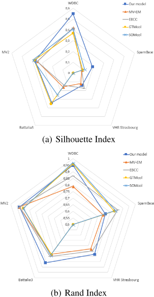
In Figure 2, we show a radar map made from the Silhouette and Rand Index tables. As one can see from the figure, our method overall outperforms the other algorithms with a much larger area coverage and we still achieve close to state of the art results with datasets for which our method is not the best one. Without surprises, the older MV-EM algorithm has the overall worst performances, followed by Kohonen maps based collaborative algorithms and then the more recent Entropy based collaborative Framework (EBCC) which sometimes has better results than our proposed method albeit with a smaller coverage area in both supervised and unsupervised indexes. Furthermore, unlike the collaborative SOM and GTM algorithms, our method does scale to relatively large dataset like VHR Strasbourg. We would like to point out that scaling is not an issue here, neither in terms of number of data nor in terms of number of features. As explained in the paper, each data can be treated separately, so a parallel run can be done. Moreover, time complexity depends on the local complexities (which are, in general, linear in the number of features). These results highlight the strength of our method, and come to back up its strong theoretical background -compared with the other competitors- with good experimental performance.
5 Conclusion
In this paper, we have proposed a new perspective on the problem of multi-source clustering. Inspired by algorithmic information theory, we reduced the problem to a model selection over a well-defined set of Turing machines. Compared to state of the art methods, our methodology is based on a wellknown theoretical background and does not rely on heuristics. Besides, its strength is highlighted by excellent experimental results both for artificial and real data, with a naive and parameter-free algorithm.
The study proposed here is just one of the various approaches to the problem. First, the properties of the designed algorithms have to be investigated from a theoretical point of view, in particular in the direction of stability. In addition, our focus was on collaborative clustering but an adaptation of our method to unsupervised ensemble learning (finding consensus) comes directly.
Acknowledgements
This research is supported by the program Futur & Ruptures (Institut Mines-T´el´ecom).
@inproceedings{ijcai2018p358,
  title     = {An Information Theory based Approach to Multisource Clustering},
  author    = {Murena, Pierre-Alexandre and Sublime, Jérémie and Matei, Basarab and Cornuéjols, Antoine},
  booktitle = {Proceedings of the Twenty-Seventh International Joint Conference on
               Artificial Intelligence, {IJCAI-18}},
  publisher = {International Joint Conferences on Artificial Intelligence Organization},
  editor    = {Jérôme Lang},
  pages     = {2581--2587},
  year      = {2018},
  month     = {7},
  note      = {Main track},
  doi       = {10.24963/ijcai.2018/358},
  url       = {https://doi.org/10.24963/ijcai.2018/358},
}
TY - CPAPER TI - An Information Theory based Approach to Multisource Clustering AU - Murena, Pierre-Alexandre AU - Sublime, Jérémie AU - Matei, Basarab AU - Cornuéjols, Antoine T2 - Proceedings of the Twenty-Seventh International Joint Conference on Artificial Intelligence, IJCAI-18 PB - International Joint Conferences on Artificial Intelligence Organization PY - 2018 SP - 2581 EP - 2587 DO - 10.24963/ijcai.2018/358 UR - https://doi.org/10.24963/ijcai.2018/358 ER -Copied
Machine-readable versions of this paper, for tools and AI agents:





