
AAR-CNNs: Auto Adaptive Regularized Convolutional Neural Networks
Proceedings of the Twenty-Seventh International Joint Conference on Artificial Intelligence. Main track. Pages 2511-2517.
https://doi.org/10.24963/ijcai.2018/348
Keywords
- Machine Learning: Neural Networks
- Machine Learning: Deep Learning
Abstract
In order to address the overfitting problem caused by the small or simple training datasets and the large model’s size in Convolutional Neural Networks (CNNs), a novel Auto Adaptive Regularization (AAR) method is proposed in this paper. The relevant networks can be called AAR-CNNs. AAR is the first method using the “abstraction extent” (predicted by AE net) and a tiny learnable module (SE net) to auto adaptively predict more accurate and individualized regularization information. The AAR module can be directly inserted into every stage of any popular networks and trained end to end to improve the networks’ flexibility. This method can not only regularize the network at both the forward and the backward processes in the training phase, but also regularize the network on a more refined level (channel or pixel level) depending on the abstraction extent’s form. Comparative experiments are performed on low resolution ImageNet, CIFAR and SVHN datasets. Experimental results show that the AAR-CNNs can achieve state-of-the-art performances on these datasets.
- [Chrabaszcz et al., 2017] Patryk Chrabaszcz, Ilya Loshchilov, and Frank Hutter. A downsampled vari- ant of imagenet as an alternative to the cifar datasets. arXiv preprint arXiv:1707.08819, 2017.
- [Deng et al., 2009] Jia Deng, Wei Dong, Richard Socher, Li- Jia Li, Kai Li, and Li Fei-Fei. Imagenet: A large-scale hierarchical image database. In Computer Vision and Pat- tern Recognition, 2009. CVPR 2009. IEEE Conference on, pages 248-255. IEEE, 2009.
- [He et al., 2016a] Kaiming He, Xiangyu Zhang, Shaoqing Ren, and Jian Sun. Deep residual learning for image recog- nition. In The IEEE Conference on Computer Vision and Pattern Recognition (CVPR), pages 770-778, June 2016.
- [He et al., 2016b] Kaiming He, Xiangyu Zhang, Shaoqing Ren, and Jian Sun. Identity mappings in deep residual networks. In European Conference on Computer Vision, pages 630-645. Springer International Publishing, 2016.
- [Hu et al., 2017] Jie Hu, Li Shen, and Gang Sun. Squeeze-and-excitation networks. arXiv preprint arXiv:1709.01507, 2017.
- [Huang et al., 2017] Gao Huang, Zhuang Liu, Kilian Q Weinberger, and Laurens van der Maaten. Densely connected convolutional networks. arXiv preprint arX- iv:1608.06993v4, 2017.
- [Ioffe and Szegedy, 2015] Sergey Ioffe and Christian Szegedy. Batch normalization: Accelerating deep net- work training by reducing internal covariate shift. In International Conference on Machine Learning, pages 448-456, 2015.
- [Krizhevsky and Hinton, 2009] Alex Krizhevsky and Geof- frey Hinton. Learning multiple layers of features from tiny images. 2009.
- [Larsson et al., 2016] Gustav Larsson, Michael Maire, and Gregory Shakhnarovich. Fractalnet: Ultra-deep neu- ral networks without residuals. arXiv preprint arX- iv:1605.07648, 2016.
- [Lee et al., 2015] Chen-Yu Lee, Saining Xie, Patrick Gal- lagher, Zhengyou Zhang, and Zhuowen Tu. Deeply- supervised nets. In Artificial Intelligence and Statistics, pages 562-570, 2015.
- [Netzer et al., 2011] Yuval Netzer, Tao Wang, Adam Coates, Alessandro Bissacco, Bo Wu, and Andrew Y Ng. Reading digits in natural images with unsupervised feature learn- ing. In NIPS workshop on deep learning and unsupervised feature learning, volume 2011, page 5, 2011.
- [Nowlan and Hinton, 1992] Steven J Nowlan and Geoffrey E Hinton. Simplifying neural networks by soft weight- sharing. Neural computation, 4(4):473-493, 1992.
- [Saad, 1998] David Saad. Online algorithms and stochastic approximations. Online Learning, 5, 1998.
- [Sermanet et al., 2012] Pierre Sermanet, Soumith Chintala, and Yann LeCun. Convolutional neural networks applied to house numbers digit classification. In Pattern Recogni- tion (ICPR), 2012 21st International Conference on, pages 3288-3291. IEEE, 2012.
- [Srivastava et al., 2014] Nitish Srivastava, Geoffrey Hinton, Alex Krizhevsky, Ilya Sutskever, and Ruslan Salakhutdi- nov. Dropout: a simple way to prevent neural networks from overfitting. Journal of Machine Learning Research, 15(1):1929-1958, 2014.
- [Sutskever et al., 2013a] Ilya Sutskever, James Martens, George Dahl, and Geoffrey Hinton. On the importance of initialization and momentum in deep learning. In Interna- tional conference on machine learning, pages 1139-1147, 2013.
- [Sutskever et al., 2013b] Ilya Sutskever, James Martens, George Dahl, and Geoffrey Hinton. On the importance of initialization and momentum in deep learning. In Interna- tional conference on machine learning, pages 1139-1147, 2013.
- [Zagoruyko and Komodakis, 2016] Sergey Zagoruyko and Nikos Komodakis. Wide residual networks. arXiv preprint arXiv:1605.07146, 2016.
References were extracted automatically from the PDF and may contain errors.
Full text extracted automatically from the PDF; figures, tables and equations may differ. The PDF is the version of record.
1 Introduction and RelatedWorks
Since the Convolutional Neural Networks (CNNs) have achieved tremendous performances at different computer vision areas, researchers have expended considerable effort designing much deeper and wider networks. However, as the increasing of the model's size, the resulting problems of vanishing gradient and overfitting have become prominent.
In order to tackle the vanishing gradient, structures with short connections between input and output are proposed. For instance, the famous ResNet [He et al., 2016a; 2016b] has achieved many breakthroughs on most of the computer vision tasks. This implies the short connections can help the gradient to flow to the preceding layers well. Moreover, an enhanced version called DenseNet is designed, which includes three dense blocks and two transition modules between two successive dense blocks. However, different from ResNet, in each dense block of DenseNet, every module has the same number of output channels and the module's input channels are concatenated with its outputs. DenseNets can get a better performance and alleviate vanishing gradient effectively.
However, these short connected models still can't combat the overfitting well when the database is simple. Therefore, FractalNet [Larsson et al., 2016], a highly generalized version of ResNet is introduced. FractalNet employs short connections and is constructed through repeatedly applying of a single expansion rule, thus, its structure is a truncated fractal. Since there are many interacting sub-paths of different lengths in FractalNet, it can be trained by dropping these paths randomly. With such regularization, co-adaptation of sub-paths can be effectively regularized in fractal architectures.
In practice, dropout [Srivastava et al., 2014] is proposed much earlier than drop-path. It is temporarily removing a neural node along with all its incoming and outgoing connections from the network with a fixed possibility. Different from drop-path, dropout can prevent co-adaptation of activations. Additionally, there are other effective regularization methods, such as weight decay [Nowlan and Hinton, 1992] and early stopping. Also, Stochastic Gradient Descent (SGD) [Saad, 1998; Sutskever et al., 2013a] is still widely utilized in the training process nowadays, which employs noisy gradients in the gradient descent. Similar to SGD, Batch Normalization [Ioffe and Szegedy, 2015] computes statistics that fluctuate with every mini-batch to regularize the network. However, Batch Normalization can reduce the effectiveness of dropout.
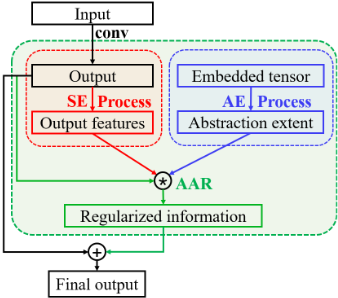
Although the above techniques are popular, they are less flexible and individualized. This paper proposes a novel AAR method. In AAR, an AE-Net first predicts its relevant stage's abstract extent. And, a learnable module (SE-Net) retrieves the channel weights according to that stage's outputs. Then, multiplying the results of AE and SE to obtain the final weights of the output from the corresponding basic module (stage). Finally, the predicted weights and the relevant output from the basic module will be multiplied again to get the final regularized information. The whole process is shown in Figure 3. The AAR method has the following advantages:
- The regularized information is obtained by predicting according to the relevant stage's abstract extent and objects' features, thus, AAR is entirely auto adaptive and more individualized.
- It can regularize the network at both the forward and the backward processes in the training phase, since it provides weights for the outputs (inferences see Section 2.4).
- It can largely improve the model's flexibility, since the regularized modules can be directly inserted into any popular networks. Moreover, they can be learned through being trained end to end.
- This method can regularize the network on a more refined level (channel or pixel level), which depends on the abstract extent's form (vector or matrix).
2 AAR-CNNs
2.1 Motivation
In order to make up the less abundant datasets, some internal augmented and regularized information can be added to the intermediate features. Meanwhile, the internal supplementary information should regularize the gradient in the back propagation process of the gradient. Moreover, Batch Normalization (BN) and SGD regularize the network on the mini-batch level, which isn't refined. Therefore, the AAR method should regularize on a more refined level (channel or level).
Additionally, since the output features from different stages have different abstract extents, the information of abstract extents is critical for the augmented information. However, designing the representations of abstract extent humanly is difficult because without enough prior and expertise knowledge. Accordingly, a randomly initialized tensor is used to represent the embedded abstract extent temporarily, then it can be transformed to obtain the final representations of abstract extent through AE-Net. This randomly initialized tensor can be seen as the learnable guided information for getting the final abstract extent. The final regularized refined level (channel or pixel level) relies on the abstract extent's form (vector or matrix). Besides this, the "Squeeze-and-Excitation" (SE) method [Hu et al., 2017] is used to retrieve the information from the different modules' objects' features to obtain more individualized regularized information. Finally, the results of AE and SE are multiplying together to obtain the weights of the output from the corresponding basic module of the backbone network. Then the predicted weights and the relevant output from the basic module will be multiplied to get the final regularized information. So the weights can regularized the network at both the forward and backward processes. In addition, since the final regularized results is obtained by the above predicting process based on the different modules' abstract extents and objects' features, the whole process is entirely auto adaptive and called AAR. The AAR can be directly inserted into each basic module of the backbone network, thus, the AAR-CNNs can be flexible and trained end to end. Moreover, all the AAR's parts (AE and SE) can also be trained by training the AAR-CNN, which implies every learnable tensor and the weights of AE and SE can be optimized automatically.
2.2 Representations of Abstract Extent
Since the convolutional receptive field is increasingly larger as the network gets deeper, the augmented information, predicted at every stage, should adjust using information of different abstract extents. In practice, the final representation's form of abstract extent should fit the size of the every stage's output. To save the memory and decrease the time consumption, an embedded low dimension tensor (matrix or vector) and two convolutional or fully connected layers are used to generate the final abstract extent's representations. Suppose x is the input of the transformation T from every basic module (e.g., residual module), then the intermediate output is y = T(x; θ) , y ∈ Rs1×s2×s3×s4 . Where, s1, s2, s3 and s4 respectively denote the mini-batch size, channels, height and width. θ is the parameters of convolutional kernels.
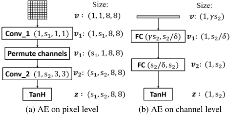
Figure 1 shows the AE process of finding representations of abstract extent. On the pixel level (Figure 1a), given the randomly initialized low dimension tensor v, v ∈ R1×1×s3×s4 . It is notable that v is a matrix and its size is equal to the relevant module's output spatial size. Two convolutional layers are utilized to project the embedded tensor to a new dimensional space. The first convolutional kernel is denoted by ω1 (ω1 ∈ R1×s1×1×1 ) and the transformational result is v1 = T (v; ω1), v1 ∈ R1×s1×s3×s4 . The first and the second dimensions of v1 will be exchanged and it becomes v1 ∈ Rs1×1×s3×s4 . After this step, another convolutional kernel indicated by ω2 (ω2 ∈ R1×s2×3×3 ) is applied and the final projected result is z = T (v1; ω2) and z ∈ Rs1×s2×s3×s4 . At last, a nonlinear T anH activation layer is attached to make the ultimate result -1 to 1. On the channel level (Figure 1b), the matrix is replaced with a vector and the convolutional layers are replaced with fully connected layers. The final representations of abstract extents can be obtained by this way. Moreover, the embedded tensor and all the parameters of linear layers can be learned and trained end to end. The entire transformation can be denoted as below:
2.3 Retrieval of Information from the Objects
Besides considering the abstract extents, object features are also critical to the final augmented information, since the found information should adapt to the different objects to make it more individualized and accurate. Accordingly, another tiny module is introduced to accomplish this goal. In order to decrease the number of parameters and also retrieve better information from the output features in the relevant module, we employ the "Squeeze-and-Excitation" (SE) method introduced in [Hu et al., 2017]. In the SE module (shown in Figure 2), a global average pooling layer is initially utilized to retrieve the features and decrease the dimensions at the same time. Then, two fully connected layers are equipped and two nonlinear activation layers (ReLu and Sigmoid) are respectively attached after them. The fully connected layer with p input nodes and q output nodes is indicated as f[p, q]. The final result is denoted as below:

where u ∈ Rs1×s2×1×1 and φ is the parameters of the fully connected layers. It is apparent that this tiny module can retrieve the global information from every channel and can be seen as a channel mask.
2.4 Obtain the Final Regularized Information
Since the abstract extents and object features have been obtained in Equations 1 and 2. A weighted mask can be got through multiplying these two parts. It can be denoted by m = z × u. At last, this weighted mask and output features are multiplied together to acquire the final regularized information, since the augmented information should be obtained under the guidance of output features. The final structure is shown in Figure 3. The augmented information will be added to the output features and the final output of every module is denoted as below:
The Regularized modules used on the pixel and channel level can be denoted by Regular - pixel(s, s2/δ) and Regular - channel(γs2, s2/δ). Where s indicates the output feature map's height or width and s2 represents the channels of the relevant basic module. From the above equation, in the forward process, the predicted augmented information is directly added to the output to supplement the feature and regularizes the network at the same time. Besides this, in the backward phase, we can obtain the gradient of every module based on Equation 3 as below:
From the above equation, the gradient is regularized in the back propagation. It can be seen as providing a filter for the original gradient. It is notable that this regularized information can provide augmented information at the forward process, meanwhile, it can also regularize the gradient at the backward process. According to the working mechanism from all the above demonstration, the networks can realize auto adaptive regularization by this proposed method.
3 Experimental Results and Analysis
3.1 Experiments on LowResolution ImageNet
Low Resolution ImageNet Datasets
The low resolution ImageNet datasets [Chrabaszcz et al., 2017] are the downsampled variants of ImageNet [Deng et al., 2009] and contain the same number of classes and images as ImageNet. There are three versions in total: ImageNet64× 64, ImageNet32×32 and ImageNet16×16. The only difference of these three versions is that the downsampled images' sizes are respectively 64 × 64, 32 × 32 and 16 × 16. Since the cost of experiments on ImageNet64 × 64 is more prohibitive than the other two datasets, and the proposed method is trying to combat the overfitting problem on small datasets, we only perform our architectures on ImageNet32 × 32 and ImageNet16×16 datasets. When the AAR-Wide ResNet (see Implementation Details) is tested, the augmentation of these two datasets keeps the same with [Chrabaszcz et al., 2017]. While for the AAR-DenseNet-BC (see Implementation Details), the datasets are only randomly horizontally flipped with probability 0.5 and do not need to be concatenated, where they will be also cropped from the images with padding 4 pixels on each side.
Implementation Details
Since our auto adaptive regularized module can be transplanted to any architectures, the final networks proposed in this paper are designed based on Wide ResNet (WRN-N-k) [Zagoruyko and Komodakis, 2016] and DenseNet-BC (DNN-g) [Huang et al., 2017] to verify the performances of AAR-CNNs. Where N indicates the depth of networks. k denotes the multiplicative factor for the number of filters of ResNet, and g denotes the growth rate. Wide ResNet has achieved better performances on many image classification tasks, whose structure is similar to ResNet, and the number of output channels at every basic module is a number of times larger than ResNet. DenseNet-BC is an extended version of Densenet with bottleneck structure, which can largely decrease the parameters and improve the parameters' efficiency. Finally, the regularized module is simply equipped at the end of each module. In the regularized modules of AAR-WRN Regular - pixel(s, s2/δ), when k is set to 10, δ is set to 16, when k is less than 10, δ is set to 8. While for the regularized modules of AAR-DN Regular - channel(γs2, s2/δ), when the g is less than 36, δ is set to 2 , otherwise, δ is set to 4. Furthermore, γ is set to 2. On ImageNet32 × 32, there are 3 blocks, therefore, the spatial size of the output feature maps at every stage is respectively 32 × 32, 16 × 16 and 8 × 8. While for ImageNet16×16, we remove the last block and the spatial size becomes 16×16 and 8×8. Finally, the embedded vector v is initialized from the normal distribution N(0, 1).
| Method | Params | Top-1 error | Top-5 error |
|---|---|---|---|
| WRN-20-2 | 0.42M | 77.00 | 54.22 |
| WRN-20-5 | 2.3M | 66.60 | 41.59 |
| WRN-20-10 | 8.9M | 59.94 | 35.10 |
| AAR-WRN-20-2 | 0.42M | 76.67 | 53.98 |
| AAR-WRN-20-5 | 2.4M | 65.52 | 40.82 |
| AAR-WRN-20-10 | 9.1M | 58.62 | 33.84 |
| DN-43-12 | 0.41M | 72.56 | 49.50 |
| DN-43-24 | 1.2M | 64.00 | 39.69 |
| DN-43-36 | 2.5M | 60.62 | 35.84 |
| DN-67-36 | 4.8M | 55.80 | 31.46 |
| DN-91-40 | 9.4M | 52.98 | 28.72 |
| AAR-DN-43-12 | 0.42M | 70.61 | 47.67 |
| AAR-DN-43-24 | 1.3M | 61.78 | 37.33 |
| AAR-DN-43-36 | 2.6M | 57.64 | 33.06 |
| AAR-DN-67-36 | 4.9M | 53.65 | 29.05 |
| AAR-DN-91-40 | 9.5M | 50.67 | 26.74 |
| Method | Params | Top-1 error | Top-5 error |
|---|---|---|---|
| WRN-28-2 | 1.6M | 56.92 | 30.92 |
| WRN-28-3 | 3.5M | 51.06 | 26.08 |
| WRN-28-5 | 9.5M | 45.46 | 21.36 |
| WRN-28-10 | 37.1M | 40.96 | 18.87 |
| AAR-WRN-28-2 | 1.6M | 55.61 | 30.02 |
| AAR-WRN-28-3 | 3.5M | 49.72 | 25.38 |
| AAR-WRN-28-5 | 9.6M | 44.11 | 20.35 |
| AAR-WRN-28-10 | 37.7M | 40.21 | 17.89 |
| DN-100-12 | 1.0M | 49.28 | 24.73 |
| DN-100-24 | 3.7M | 42.03 | 18.70 |
| DN-100-36 | 7.8M | 38.52 | 16.27 |
| DN-100-40 | 9.5M | 38.34 | 16.18 |
| AAR-DN-100-12 | 1.1M | 47.64 | 23.10 |
| AAR-DN-100-24 | 3.8M | 39.46 | 17.05 |
| AAR-DN-100-36 | 7.9M | 37.43 | 16.10 |
| AAR-DN-100-40 | 9.6M | 36.81 | 15.04 |
The almost identical weight initialization and optimization configuration introduced in Wide ResNet and DenseNet-BC are adopted in AAR-WRN and AAR-DN. But the mini-batch size is set to 100. The training epoches are set to 40 and 80 and utilizes the SGD method and Nesterov momentum [Sutskever et al., 2013b] to optimize. The optimization starts from the initial learning rate with 0.01 and 0.1, which is respectively divided by 5 every 10 epoches and divided by 10 at 50% and 75% of the total number of training epochs. The momentum is 0.9, and the weight decay is respectively set to 5e - 4 and 1e - 4 on AAR-WRN and AAR-DN.
Experimental Results
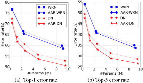
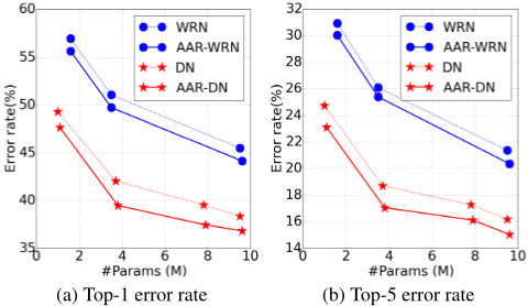
In order to verify the effectiveness of the AAR module, the error rates are shown in Figure 4 and 5. It is noted that the models with the AAR modules all achieve better performances than the relevant traditional architectures on these two datasets. Compared with AAR-WRNs (reported in
| Method | Depths | Params | CIFAR-10 | CIFAR-100 |
|---|---|---|---|---|
| FractalNet (dropout/drop-path) ( in [Larsson et al., 2016]) | 21 | 38.6M | 4.60 | 23.73 |
| ResNet (pre-activation) ( in [Huang et al., 2017]) | 1001 | 10.2M | 4.62 | 22.71 |
| Wide ResNet ( in [Zagoruyko and Komodakis, 2016]) | 28 | 36.5M | 4.17 | 20.50 |
| DN-100-12 (in [Huang et al., 2017] ) | 100 | 0.8M | 4.51 | 22.27 |
| DN-190-40 (in [Huang et al., 2017] ) | 190 | 25.6M | 3.46 | 17.18 |
| AAR-DN-100-12 (ours ) | 100 | 0.8M | 4.00 | 20.77 |
| AAR-DN-190-40 (ours ) | 190 | 26.1M | 3.28 | 17.02 |
[Chrabaszcz et al., 2017]), the way of dense connections leads to the more efficiency of ARR-DNs' parameters. The final experimental results of all the contrastive models are shown in Table 1 and Table 2. For AAR-WRNs, on ImgeNet16×16, AAR-WRN-20-10 respectively achieves the best top-1 and top-5 error rates 58.62% and 33.84%. On ImgeNet32 × 32, AAR-WRN-28-10 also respectively achieves the best top1 and top-5 error rates 40.21% and 17.89%. While for AAR-DNs, it is significant that they largely decrease the error rates and achieve state-of-the-art performances. For example, AAR-DN-91-40 deceases the top-1 and top-5 error rates by 9.27% and 8.36% compared with WRN-20-10 on ImgeNet16 × 16. Also, AAR-DN-100-40 deceases the top1 and top-5 error rates by 4.15% and 3.83% compared with WRN-28-10 on ImgeNet32 × 32. This implies the AAR method can significantly improve the performances of classical models.
3.2 Experiments on CIFAR
CIFAR Datasets
CIFAR [Krizhevsky and Hinton, 2009] datasets include CIFAR-10 and CIFAR-100. They both have 60, 000 32 × 32pixel colored nature scene images in total, including 50, 000 images for training and 10, 000 images for testing in 10 and 100 classes. Data augmentation is the same with the common practice in [Huang et al., 2017].
Networks and Initialization
Since DenseNet-BC can achieve much better performances on CIFAR datasets [Huang et al., 2017], we implement the AAR-DNs based on it. The AAR-DNs are the same with the networks on ImageNet32 × 32. They employ Regular - channel(γg, g/δ), where g denotes the growth rate [Huang et al., 2017]. γ is set to 2, and δ is respectively set to 2 and 4 when g is 12 and 40. The embedded vector v is respectively randomly initialized for normal distribution N(0, 0.012 ) and N(0, 1) on CIFAR-10 and CIFAR-100. AAR-DNs also utilize the same weight initialization and optimization configuration introduced in DenseNet-BC [Huang et al., 2017].
Experimental Results
The final results are shown in Table 3. Compared with DN-100-12, the AAR-DN-100-12 decreases the error rates by 0.51% and 1.50% on these two datasets with almost the same parameters (0.8M). Especially, AAR-DN-190-40 also achieves the state-of-the-art results with 3.28% and 17.02% error rates on CIFAR-10 and CIFAR-100, respectively.
| Method | Params | Error rate |
|---|---|---|
| DN-100-12 (in [Huang et al., 2017] ) | 0.8M | 1.76 |
| DN-250-24 (in [Huang et al., 2017] ) | 15.3M | 1.74 |
| AAR-DN-100-12 (ours ) | 0.8M | 1.71 |
| AAR-DN-70-24 (ours ) | 2.0M | 1.66 |
3.3 Experiments on SVHN
SVHN Datasets
The Street View House Numbers (SVHN) dataset [Netzer et al., 2011] includes 73,257 training images, 26,032 testing images and 531,131 images for additional training. They are all 32 × 32 colored digit images. The preprocess of SVHN is the same with [Sermanet et al., 2012; Lee et al., 2015; Huang et al., 2017].
Networks and Initialization
Similar to Densenet-BC, we implement the AAR-DNs based on it. Since this dataset is very simple, AAR-DNs employ Regular -pixel(s, g/2) to regularize on the pixel level, and s is respectively set to 32, 16 and 8 at three dense blocks. At last, v is randomly initialized for normal distribution N(0, 1). AAR-DNs utilize the same weight initialization and optimization configuration introduced in DenseNet-BC [Huang et al., 2017] on SVHN. However, the technique dropout is not utilized in AAR-DNs.
Experimental Results
Table 4 gives the final error rate of SVHN compared with DenseNet-BC, it is apparent that our AAR-DNs obtain better performances. In particular, AAR-DN-70-24 decreases the error rate efficiently by utilizing much less parameters than DN-250-24 (2.0M vs 15.3M). The results imply the effectiveness of the AAR method.
3.4 Further Investigation of AARMethod
In order to further verify the performance of the AAR module, the AAR module only using SE or AE is equipped in the WRN-28-k and the corresponding model is indicated by SEWRN or AE-WRN. The comparisons of these models' performances are listed in Table 5. From the results, it is apparent that almost all the SE-WRNs and AE-WRNs can improve the performance than WRNs. It verifies the effectiveness of SE and AE, that is to say, the different objects' features and the abstract extents are both critical to the final predicted regularized information. However, the AAR-WRNs employing the combination of SE and AE can make a larger improvement of the performance and achieve the best results than the other models. Accordingly, it can prove that using both the SE and AE in AAR is necessary to predict more individualized and accurate regularized information.
| Top-1 error | Top-5 error | |||||
|---|---|---|---|---|---|---|
| k = 2 | k = 3 | k = 5 | k = 2 | k = 3 | k = 5 | |
| WRN | 56.92 | 51.06 | 45.46 | 30.92 | 26.08 | 21.36 |
| SE-WRN | 56.89 | 51.03 | 45.02 | 31.28 | 25.76 | 21.00 |
| AE-WRN | 56.73 | 50.87 | 44.44 | 31.22 | 25.82 | 20.74 |
| AAR-WRN | 55.61 | 49.72 | 44.11 | 30.02 | 25.38 | 20.35 |
3.5 Effects on Filters' Relationships
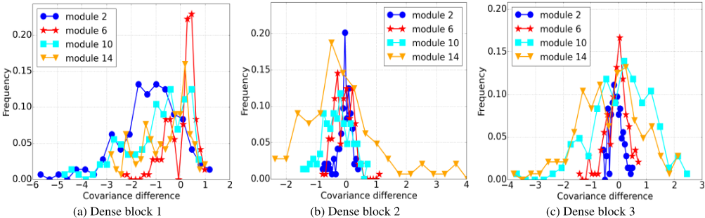
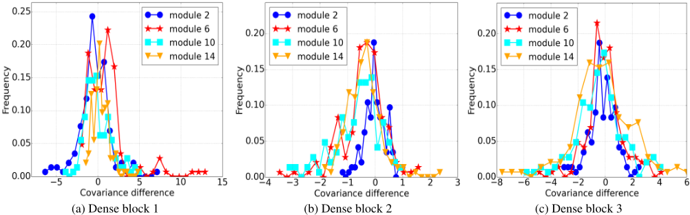
A further investigation of regularized information is made through calculating the covariances of adjacent convolutional layers' output feature maps, which shows the filters' relationships between adjacent convolutional layers. The smaller the covariance, the sparser the filters are. The covariance differences of filters before and after regularization by the AAR method are computed to investigate the effects on filters' relationships. Figure 6 shows the frequency of the final results of AAR-DN-100-12 on ImageNet32×32 and CIFAR-10, because on these two datasets, the performing networks have almost the same structure settings. Since this network has 3 big dense blocks, and in each dense block, there are 16 basic modules. In order to illustrate the changing trend, we select 4 modules (2nd , 6th , 10th and 14th ) to represent the different stages at each dense block and plot the results.
From Figure 6, it is apparent that the first dense block's (Figure 6a) covariance differences mostly distribute the part of less than 0. It implies the regularized information decreases the filters relationships. In other words, it tends to force the filters to be much sparser at the first stage of the networks to make every small filter learn features separatively, which can adapt to the richness of categories. However, with the increasing of depth, it seems that the AAR method tries to decrease the sparsity ability leading to obtaining more structured information. By contrast, from the Figure 7, the regularization information force the filters to be denser on the low abstract level and sparser on the high abstract level. This is most probably because CIFAR-10 is much smaller and simpler than ImageNet32×32, therefore, it suggests only the first stage of the network can catch almost adequate structured features through enhancing the relationships appropriately, then the filters of the other stages are forced sparser to avoid overfitting. All the experimental results indicate the regularized information found by the AAR method is more individualized to auto adaptively adjust the filters sparsity based on the properties of networks and objects' features, which can effectively combat the overfitting problem when facing small and simple datasets. Meanwhile, this method also improves the flexibility of the networks significantly.
4 Conclusion
This paper proposes a novel auto adaptive regularized module to explicitly find much more appropriate regularization information for CNNs. Compared with other regularization methods, the AAR method is the first utilizing the information of abstract extents at different stages and specific objects from every mini-batch to predict more individualized regularization information. The AAR modules can be easily inserted into any classical CNNs and trained end to end, which leads to significantly improving the model's flexibility. It can also regularize the network at both the forward and the backward processes in the training phase. The AAR-CNNs are tested on down-sampled ImageNet, CIFAR and SVHN datasets. Experimental results show that the AAR-CNNs can significantly improve the performances of the models and address the overfitting problem effectively when facing simple datasets.
Acknowledgments
This work is supported by NSFC fund (61332011), Shenzhen Fundamental Research fund (JCYJ20170811155442454), and Medical Biometrics Perception and Analysis Engineering Laboratory, Shenzhen, China.
@inproceedings{ijcai2018p348,
  title     = {AAR-CNNs: Auto Adaptive Regularized Convolutional Neural Networks},
  author    = {Lu, Yao and Lu, Guangming and Xu, Yuanrong and Zhang, Bob},
  booktitle = {Proceedings of the Twenty-Seventh International Joint Conference on
               Artificial Intelligence, {IJCAI-18}},
  publisher = {International Joint Conferences on Artificial Intelligence Organization},
  editor    = {Jérôme Lang},
  pages     = {2511--2517},
  year      = {2018},
  month     = {7},
  note      = {Main track},
  doi       = {10.24963/ijcai.2018/348},
  url       = {https://doi.org/10.24963/ijcai.2018/348},
}
TY - CPAPER TI - AAR-CNNs: Auto Adaptive Regularized Convolutional Neural Networks AU - Lu, Yao AU - Lu, Guangming AU - Xu, Yuanrong AU - Zhang, Bob T2 - Proceedings of the Twenty-Seventh International Joint Conference on Artificial Intelligence, IJCAI-18 PB - International Joint Conferences on Artificial Intelligence Organization PY - 2018 SP - 2511 EP - 2517 DO - 10.24963/ijcai.2018/348 UR - https://doi.org/10.24963/ijcai.2018/348 ER -Copied
Machine-readable versions of this paper, for tools and AI agents:





