
Exact Low Tubal Rank Tensor Recovery from Gaussian Measurements
Proceedings of the Twenty-Seventh International Joint Conference on Artificial Intelligence. Main track. Pages 2504-2510.
https://doi.org/10.24963/ijcai.2018/347
Keywords
- Machine Learning: Feature Selection ; Learning Sparse Models
- Computer Vision: Statistical Methods and Machine Learning
Abstract
The recent proposed Tensor Nuclear Norm (TNN) [Lu et al., 2016; 2018a] is an interesting convex penalty induced by the tensor SVD [Kilmer and Martin, 2011]. It plays a similar role as the matrix nuclear norm which is the convex surrogate of the matrix rank. Considering that the TNN based Tensor Robust PCA [Lu et al., 2018a] is an elegant extension of Robust PCA with a similar tight recovery bound, it is natural to solve other low rank tensor recovery problems extended from the matrix cases. However, the extensions and proofs are generally tedious. The general atomic norm provides a unified view of low-complexity structures induced norms, e.g., the l1-norm and nuclear norm. The sharp estimates of the required number of generic measurements for exact recovery based on the atomic norm are known in the literature. In this work, with a careful choice of the atomic set, we prove that TNN is a special atomic norm. Then by computing the Gaussian width of certain cone which is necessary for the sharp estimate, we achieve a simple bound for guaranteed low tubal rank tensor recovery from Gaussian measurements. Specifically, we show that by solving a TNN minimization problem, the underlying tensor of size n1×n2×n3 with tubal rank r can be exactly recovered when the given number of Gaussian measurements is O(r(n1+n2−r)n3). It is order optimal when comparing with the degrees of freedom r(n1+n2−r)n3. Beyond the Gaussian mapping, we also give the recovery guarantee of tensor completion based on the uniform random mapping by TNN minimization. Numerical experiments verify our theoretical results.
- [Amelunxen et al., 2014] Dennis Amelunxen, Martin Lotz, Michael B McCoy, and Joel A Tropp. Living on the edge: Phase transitions in convex programs with random data. Information and Inference, pages 224-294, 2014.
- [Candès and Recht, 2009] E.J. Candès and B. Recht. Exact matrix completion via convex optimization. Foundations of Computational mathematics, 9(6):717-772, 2009.
- [Candès et al., 2006] Emmanuel J Candès, Justin Romberg, and Terence Tao. Robust uncertainty principles: Exact signal reconstruction from highly incomplete frequency information. TIT, 52(2):489-509, 2006.
- [Chandrasekaran et al., 2012] Venkat Chandrasekaran, Ben- jamin Recht, Pablo A Parrilo, and Alan S Willsky. The convex geometry of linear inverse problems. Foundations of Computational mathematics, 12(6):805-849, 2012.
- [Chen, 2015] Yudong Chen. Incoherence-optimal matrix completion. TIT, 61(5):2909-2923, May 2015.
- [Donoho and Tanner, 2009] David Donoho and Jared Tanner. Counting faces of randomly projected polytopes when the projection radically lowers dimension. Journal of the Amer- ican Mathematical Society, 22(1):1-53, 2009.
- [Foygel and Mackey, 2014] Rina Foygel and Lester Mackey. Corrupted sensing: Novel guarantees for separating struc- tured signals. TIT, 60(2):1223-1247, 2014.
- [Kilmer and Martin, 2011] Misha E Kilmer and Carla D Mar- tin. Factorization strategies for third-order tensors. Linear Algebra and its Applications, 435(3):641-658, 2011.
- [Lu et al., 2015] Canyi Lu, Changbo Zhu, Chunyan Xu, Shuicheng Yan, and Zhouchen Lin. Generalized singu- lar value thresholding. In AAAI, 2015.
- [Lu et al., 2016] Canyi Lu, Jiashi Feng, Yudong Chen, Wei Liu, Zhouchen Lin, and Shuicheng Yan Yan. Tensor robust principal component analysis: Exact recovery of corrupted low-rank tensors via convex optimization. In CVPR. IEEE, 2016.
- [Lu et al., 2018a] Canyi Lu, Jiashi Feng, Yudong Chen, Wei Liu, Zhouchen Lin, and Shuicheng Yan Yan. Tensor robust principal component analysis with a new tensor nuclear norm. arXiv preprint arXiv:1804.03728, 2018.
- [Lu et al., 2018b] Canyi Lu, Jiashi Feng, Shuicheng Yan, and Zhouchen Lin. A unified alternating direction method of multipliers by majorization minimization. TPAMI, 40(3):527-541, 2018.
- [Mu et al., 2014] Cun Mu, Bo Huang, John Wright, and Don- ald Goldfarb. Square deal: Lower bounds and improved relaxations for tensor recovery. In ICML, pages 73-81, 2014.
- [Recht et al., 2010] Benjamin Recht, Maryam Fazel, and Pablo A Parrilo. Guaranteed minimum-rank solutions of lin- ear matrix equations via nuclear norm minimization. SIAM review, 52(3):471-501, 2010.
- [Zhang and Aeron, 2017] Zemin Zhang and Shuchin Aeron. Exact tensor completion using t-SVD. TSP, 65(6):1511- 1526, 2017.
References were extracted automatically from the PDF and may contain errors.
Full text extracted automatically from the PDF; figures, tables and equations may differ. The PDF is the version of record.
1 Introduction
Many engineering problems look for solutions to underdetermined systems of linear equations: a system is considered underdetermined if there are fewer equations than unknowns.
∗Corresponding author.
Suppose we are given information about an object x0 ∈ Rd of the form Φx0 ∈ Rm where Φ is an m × d matrix. We want the bound on the number of rows m to ensure that x0 is the unique minimizer to the problem
Here ‖·‖A is a norm with some suitable properties which encourage solutions to conform to some notion of simplicity. For example, the compressed sensing problem aims to recover a sparse vector x0 from (1) by taking ‖·‖A as the ℓ1-norm ‖x‖1. We would like to know that how many measurements are required to recover an s-sparse x0. This of course depends on the kind of measurements. For instance, it is shown in [Cand`es et al., 2006] that 20s log d randomly selected Fourier coefficients are sufficient. If the Gaussian measurement map (Φ has entries i.i.d. sampled from a Gaussian distribution with mean 0 and variance 1m ) is used, 2s log ds + 54 s measurements are needed [Donoho and Tanner, 2009; Chandrasekaran et al., 2012]. Another interesting structured object is the low-rank matrix X0 ∈ Rn1×n2 . In this case, the ith component of a linear operator is given by [Φ(X0)]i = 〈Φi,X0〉, where Φi ∈ Rn1×n2 . This includes the matrix completion problem [Cand`es and Recht, 2009] as a special case based on a proper choice of Φi. By taking ‖·‖A as the matrix nuclear norm ‖X‖∗, the convex program (1) recovers X0 provided that the number of measurements is of the order µ(X0)r(n1 + n2 - r) log2 (n1 + n2), where r is the rank of X0 and µ(X0) is the incoherence parameter [Cand`es and Recht, 2009; Chen, 2015]. Compared with the degrees of freedom r(n1 + n2 - r) of the rank-r matrix, such a rate is optimal (up to a logarithmic factor). If the Gaussian measurement map is used, about 3r(n1 +n2 - r) samples are sufficient for exact recovery [Recht et al., 2010].
Beyond the sparse vector and low-rank matrix, there have some other structured signals which can be recovered by (1). The work [Chandrasekaran et al., 2012] gives some more examples, presents a unified view of the convex programming to inverse problems and provides a simple framework to derive exact recovery bounds for a variety of simple models. Their considered models are formed as the sum of a few atoms from some elementary atomic sets. The convex programming formulation is based on minimizing the norm induced by the convex hull of the atomic set; this norm is referred to as the atomic norm (the ℓ1-norm and nuclear norm are special cases). By using the properties of the atomic norm, an analysis of the underlying convex geometry provides sharp estimates of the number of generic measurements required for exact recovery of models from partial information. A key step to estimate the required number of measurements is to compute the Gaussian width of the tangent cone associated with the atomic norm ball.
This work focuses the study on the low-rank tensor which is an interesting object structured that has many applications in signal processing. Recovering low-rank tensor is not easy since the tensor rank is not well defined. There have several tensor rank definitions, but each has its limitation. For example, the CP rank, defined as the smallest number of rank one tensor decomposition, is generally NP hard to compute. Also, its convex envelope is in general intractable. The tractable Tucker rank is more widely used. However, considering the low Tucker rank tensor recovery problem, the required number of measurements of existing convex model is much higher than the degrees of freedom [Mu et al., 2014]. This is different from the nuclear norm minimization for low-rank matrix recovery which has order optimal rate [Chen, 2015].
In this work, we first study the low tubal rank tensor recovery from Gaussian measurements. Tensor RPCA [Lu et al., 2016; 2018a] studies the low tubal rank tensor recovery from sparse corruptions by Tensor Nuclear Norm (TNN) minimization. We show that TNN is a new instance of the atomic norm based on a proper choice of the atomic set. From the perspective of atomic norm minimization, we give the low tubal rank recovery guarantee from Gaussian measurements. Specifically, to recover a tensor of size n1×n2×n3 with tubal rank r from Gaussian measurement by TNN minimization, the required number of measurements is O(r(n1 +n2 -r)n3). It is order optimal when comparing with the degrees of freedom r(n1 + n2 - r)n3. Second, we study the tensor completion problem from uniform random sampling. We show that, to recover a tensor of tubal rank r, the sampling complexity is O(r min(n1, n2)n3 log2 (min(n1, n2)n3)), which is order optimal (up to a log factor). The same problem has been studied in [Zhang and Aeron, 2017] but its proofs have several errors.
2 Notations and Preliminaries
We introduce some notations used in this paper. We denote tensors by boldface Euler script letters, e.g., A, matrices by boldface capital letters, e.g., A, vectors by boldface lowercase letters, e.g., a, and scalars by lowercase letters, e.g., a. We denote In as the n × n sized identity matrix. The field of real number and complex number are denoted as R and C, respectively. For a 3-way tensor A ∈ Cn1×n2×n3 , we denote its (i, j, k)-th entry as Aijk or aijk and use the Matlab notation A(i, :, :), A(:, i, :) and A(:, :, i) to respectively denote the i-th horizontal, lateral and frontal slice. More often, the frontal slice A(:, :, i) is denoted compactly as A(i) . The tube is denoted as A(i, j, :). The inner product of A and B in Cn1×n2 is defined as 〈A,B〉 = Tr(A∗B), where A∗ denotes the conjugate transpose of A and Tr(·) denotes the matrix trace. The inner product of A and B in Cn1×n2×n3 is defined as 〈A,B〉 = ∑n3 i=1 〈A(i) ,B(i)〉. For any A ∈ Cn1×n2×n3 , the complex conjugate of A is denoted as conj(A), which takes the complex conjugate of all entries of A. We denote ⌊t⌋ as the nearest integer less than or equal to t and ⌈t⌉ as the one greater than or equal to t. We denote the ℓ1-norm as ‖A‖1 = ∑ijk |aijk|, the infinity norm as ‖A‖∞ = maxijk |aijk| and the Frobenius norm as ‖A‖F = √∑ijk |aijk|2 . The same norms are used for matrices and vectors. The spectral norm of a matrix A is denoted as ‖A‖ = maxi σi(A), where σi(A)'s are the singular values of A. The matrix nuclear norm is ‖A‖∗ = ∑i σi(A).
For A ∈ Rn1×n2×n3 , by using the Matlab command fft, we denote ¯ A ∈ Cn1×n2×n3 as the result of Fast Fourier Transformation (FFT) of A along the 3-rd dimension, i.e., ¯ A = fft(A, [ ], 3). In the same fashion, we can compute A from ¯ A using the inverse FFT, i.e., A = ifft( ¯ A, [ ], 3) . In particular, we denote ¯ A as a block diagonal matrix with i-th block on the diagonal as the frontal slice ¯ A(i) of ¯ A, i.e.,
The block circulant matrix of A is defined as
The block circulant matrix can be block diagonalized, i.e.,
where Fn3 ∈ Cn3×n3 is the discrete Fourier transformation matrix, ⊗ denotes the Kronecker product. Note that (Fn3 ⊗ In1 )/√n3 is orthogonal. We define the following operators
Definition 1. (t-product) [Kilmer andMartin, 2011] Let A ∈ Rn1×n2×n3 and B ∈ Rn2×l×n3 . Then the t-product A ∗ B is defined to be a tensor C ∈ Rn1×l×n3 ,
The frontal slices of ¯ A has the following property
Using the above property, the work [Lu et al., 2018a] proposes a more efficient way for computing t-product than the method in [Kilmer and Martin, 2011].
Definition 2. (Conjugate transpose) [Lu et al., 2016; 2018a] The conjugate transpose of a tensor A of size n1 × n2 × n3 is the n2 × n1 × n3 tensor A∗ obtained by conjugate transposing each of the frontal slice and then reversing the order of transposed frontal slices 2 through n3.
Definition 3. (Identity tensor) [Kilmer and Martin, 2011] The identity tensor I ∈ Rn×n×n3 is the tensor whose first frontal slice is the n × n identity matrix, and other frontal slices are all zeros.
Definition 4. (Orthogonal tensor) [Kilmer and Martin, 2011] A tensor Q ∈ Rn×n×n3 is orthogonal if it satisfies
Definition 5. (F-diagonal Tensor) [Kilmer and Martin, 2011] A tensor is called f-diagonal if each of its frontal slices is a diagonal matrix.
Theorem 1. (T-SVD) [Lu et al., 2018a; Kilmer and Martin, 2011] Let A ∈ Rn1×n2×n3 . Then it can be factored as
where U ∈ Rn1×n1×n3 , V ∈ Rn2×n2×n3 are orthogonal, and S ∈ Rn1×n2×n3 is a f-diagonal tensor.
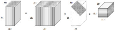
Theorem 1 gives the t-SVD based on t-product. See Figure 1 for an illustration. Theorem 1 appears first in [Kilmer and Martin, 2011] but their proof is not rigorous since it cannot guarantee that U and V are real tensors. The work [Lu et al., 2018a] fixes this issue by using property (2), and further gives a more efficient way for computing t-SVD (see Algorithm 1). Algorithm 1 only needs to compute ⌈ n3+1 2 ⌉ matrix SVDs, while this number is n3 by the method in [Kilmer and Martin, 2011]. The entries of the first frontal slice S(:, :, 1) are called as the singular values of the tensor A. The number of nonzero singular values is equivalent to the tensor tubal rank.
Definition 6. (Tensor tubal rank) [Lu et al., 2018a] ForA ∈ Rn1×n2×n3 , the tensor tubal rank, denoted as rankt(A), is defined as the number of nonzero singular values of cS, where S is from the t-SVD of A = U ∗ S ∗ V ∗ . We can write
For A ∈ Rn1×n2×n3 with tubal rank r, it has the skinny t-SVD, i.e., A = U ∗ S ∗ V ∗ , where U ∈ Rn1×r×n3 , S ∈ Rr×r×n3 , and V ∈ Rn2×r×n3 , in which U ∗ ∗ U = I and V ∗ ∗ V = I. We use the skinny t-SVD throughout this paper.
Definition 7. (Tensor nuclear norm) [Lu et al., 2018a] Let A = U ∗S ∗V ∗ be the t-SVD of A ∈ Rn1×n2×n3 . The tensor nuclear norm of A is defined as the sum of the tensor singular values, i.e., ‖A‖∗ = ∑ri=1 S(i, i, 1), where r = rankt(A).
Algorithm 1 T-SVD
Input: A ∈ Rn1×n2×n3 .
Output: T-SVD components U, S and V of A.
- Compute ¯ A = fft(A, [ ], 3).
- Compute each frontal slice of ¯ U, ¯ S and ¯V from ¯ A by for i = 1, · · · , ⌈ n3+1 2 ⌉ do [ ¯U (i) , ¯ S(i) , ¯ V (i) ] = SVD( ¯ A(i) );
end for
end for
The above definition of TNN is defined based on t-SVD. It is equivalent to 1 n3 ‖ ¯ A‖∗ as given in [Lu et al., 2016]. Indeed,
Above the factor 1 n3 is from the property ‖Fn3 ‖2F = n3, where Fn3 is the discrete Fourier transformation matrix.
Definition 8. (Tensor spectral norm) [Lu et al., 2016] The tensor spectral norm of A ∈ Rn1×n2×n3 , denoted as ‖A‖, is defined as ‖A‖ = ‖bcirc(A)‖.
TNN is the dual norm of the tensor spectral norm, and vice versa. Definite the tensor average rank as ranka(A) = 1 n3 bcirc(A). Then the convex envelope of the tensor average rank is the tensor nuclear within the set {A|‖A‖ ≤ 1}. It is worth mentioning that the above definition of tensor nuclear norm is different from the one in [Zhang and Aeron, 2017] due to the factor 1 n3 . This factor is crucial in theoretical analysis. Intuitively, it makes the model, theoretical proof and the way for optimization consistent with the matrix cases.
3 Tensor Nuclear Norm Is an Atomic Norm
Based on the above tensor tubal rank, this work considers the following problem. Suppose that we have a linear map Φ : Rn1×n2×n3 → Rm and the observations y = Φ(M) forM∈ Rn1×n2×n3 which has tubal rank r. Our goal is to recover the underlyingMfrom the observations y. This can be achieved by solving the following convex program
Now, how many measurements are required to guarantee the exact recovery (i.e., ˆX =M)? This problem is an extension of the low-rank matrix recovery problem [Recht et al., 2010].
To answer the above question, we will use the unified theory in [Chandrasekaran et al., 2012] which provides sharp estimates of the number of measurements required for exact and robust recovery of models from Gaussian measurements. The key challenge is to reformulate TNN as a special case of the atomic norm and compute the Gaussian width. In this section, we will show that TNN is a special case of the atomic norm.
Let A be a collection of atoms that is a compact subset of Rp and conv(A) be its convex hull. The atomic norm induced by A is defined as [Chandrasekaran et al., 2012]
We also need some other notations which will be used in the analysis. The support function of A is given as
If ‖·‖A is a norm, the support function ‖·‖∗A is the dual norm of this atomic norm.
A convex set C is a cone if it is closed under positive linear combinations. The polar C ∗ of a cone C is the cone
The tangent cone at nonzero x is defined as
The normal cone NA(x) at x is defined as
Note that the normal cone NA(x) is the conic hull of the subdifferential of the atomic norm at x.
By a proper choice of the set A, the atomic norm reduces to several well-known norms. For example, let A ⊂ Rp be the set of unit-norm one-sparse vectors {±ei}pi=1 . Then k-sparse vectors in Rp can be constructed using a linear combination of k elements of the atomic set and the atomic norm ‖x‖A reduces to the ℓ1-norm. Let A be the set of rank-one matrices of unit-Euclidean-norm. Then the rank-k matrices can be constructed using a linear combination of k elements of the atomic set and the atomic norm reduces to the matrix nuclear norm. Some other examples of atomic norms can be found in [Chandrasekaran et al., 2012]. At the following, we define a new atomic set A, and show that TNN is also an atomic norm induced by such an atomic set.
Let D be a set of the following matrices, i.e., D ∈ D where
where Di ∈ Cn1×n2 and there exists k such that Dk ̸= 0, rank(Dk) = 1, ‖Dk‖F = 1, and Dj = 0, for all j ̸= k. Then, for any A ∈ Rn1×n2×n3 , we have
.
Above we use the property of the rank one matrix decomposition of a matrix. This is equivalent to
where (4) uses the linear property of the inverse discrete Fourier transformation along the third dimension of a three way tensor. Motivated by (4), we define the atomic set A as
Theorem 2. Let A be the set defined as in (5). The atomic norm ‖A‖A is TNN, i.e.,
For any W ∈ A, we have ‖W‖∗ = n3‖D‖∗ = ‖ ¯D‖∗ = 1. So the convex hull conv(A) is the TNN ball in which TNN is less than or equal to one. Interpreting TNN as a special atomic norm by choosing a proper atomic set is crucial for the low-rank tensor recovery guarantee.
4 Low-rank Tensor Recovery fromGaussian Measurements
The Corollary 3.3 in [Chandrasekaran et al., 2012] shows that x0 is the unique solution to problem (1) with high probability provided m ≥ ω2 (TA(x0) ∩ Sp-1 ) + 1. Here, TA(x0) is the tangent cone at x0 ∈ Rp , Sp-1 is the unit sphere, and ω(S) is the Gaussian width of a set S, defined as
where g is a vector of independent zero-mean unit-variance Gaussians. To apply such a result for our low tubal rank recovery, we need to estimate the Gaussian width of our atomic set A defined in (5).
Theorem 3. LetM∈ Rn1×n2×n3 be a tubal rank r tensor and A in (5). We have that
Now, by using (6) and the Corollary 3.3 in [Chandrasekaran et al., 2012], we have the following main result.
Theorem 4. Let Φ : Rn1×n2×n3 → Rn be a random map with i.i.d. zero-mean Gaussian entries having variance 1m and M∈ Rn1×n2×n3 be a tensor of tubal rank r. Then, with high probability, we have:
- exact recovery: ˆX = M, where ˆX is the unique optimum of (3), provided that m ≥ 3r(n1 + n2 - r)n3 + 1;
(2) robust recovery: ‖ ˆX -M‖F ≤ 2δ ϵ , where ˆX is optimal
The above theorem shows that the tensor with tubal rank r can be recovered exactly by solving the convex program (3) or approximately by (7) when the required number of measurements is of the order O(r(n1 +n2 -r)n3). Note that such a rate is optimal compared with the degrees of freedom of a tensor with tubal rank r.
Theorem 5. A n1 × n2 × n3 sized tensor with tubal rank r has at most r(n1 + n2 - r)n3 degrees of freedom.
It is worth mentioning that the guarantee for low tubal rank tehsor recovery in Theorem 4 is an extension of the low matrix guarantee in [Recht et al., 2010; Chandrasekaran et al., 2012]. If n3 = 1, the tensor X reduces to a matrix, the tensor tubal rank reduces to the matrix rank, and TNN reduces to the matrix nuclear norm. Thus the convex program (3) and the theoretical guarantee in Theorem 4 include the low rank matrix recovery model and guarantee as special cases, respectively. Compared with the existing low rank tensor recovery guarantees (based on different tensor ranks, e.g., [Mu et al., 2014]) which are not order optimal, our guarantee enjoys the same optimal rate as the matrix case and our model (3) is computable.
5 Exact Tensor Completion Guarantee
Theorem 4 gives the recovery guarantee of program (3) based on the Gaussian measurements. In this section, we consider the tensor completion problem which is a special case of (3) but based on the uniform random mapping. Suppose that M ∈ Rn1×n2×n3 and rankt(M) = r. We consider the Bernoulli model in this work: the entries of M are independently observed with probability p. We denote the set of the indices of the observed entries as Ω. We simply denote Ω ∼ Ber(p). Then, the tensor completion problem asks for recovering M from the observations {Mij , (i, j, k) ∈ Ω}. We can solve this problem by solving the following program
where PΩ(X) denotes the projection of X on the observed set Ω. The above model extends the matrix completion task by convex nuclear norm minimization [Cand`es and Recht, 2009]. To guarantee the exact recovery, we need the following tensor incoherence conditions [Lu et al., 2018a]
where˚ei denotes the tensor column basis, which is a tensor of size n × 1 × n3 with its (i, 1, 1)-th entry equaling 1 and the rest equaling 0. We also define the tensor tube basis ˙ek, which is a tensor of size 1×1×n3 with its (1, 1, k)-th entry equaling 1 and the rest equaling 0. Denote n(1) = max(n1, n2) and n(2) = min(n1, n2).
| r = rankt(X0) = 0.2n | ||||
|---|---|---|---|---|
| n | rankt(X0) | m | rankt( ˆX) | ‖ ˆX-X0‖F ‖X0‖F |
| 10 | 2 | 541 | 2 | 1.2e-9 |
| 20 | 4 | 2161 | 4 | 1.6e-9 |
| 30 | 6 r | 4861 | 6 | 1.5e-9 |
| = rankt(X0) = 0.3n | ||||
| n | rankt(X0) | m | rankt( ˆX) | ‖ ˆX-X0‖F ‖X0‖F |
| 10 | 3 | 766 | 3 | 1.6e-9 |
| 20 | 6 | 3061 | 6 | 1.2e-9 |
| 30 | 9 | 6886 | 9 | 1.2e-9 |
Theorem 6. LetM∈ Rn1×n2×n3 with rankt(M) = r and the skinny t-SVD be M = U ∗ S ∗ V ∗ . Suppose that the indices Ω ∼ Ber(p) and the tensor incoherence conditions (9)-(10) hold. There exist universal constants c0, c1, c2 > 0 such that if
thenMis the unique solution to (8) with probability at least 1 - c1(n1 + n2)-c2 .
Theorem 6 shows that, to recover a n1 × n2 × n3 sized tensor with tubal rank r, the sampling complexity is O(rn(1)n3 log2 (n(1)n3)). Such a bound is tight compared with the degrees of freedom 1 .
6 Experiments
In this section, we conducts experiments to first verify the exact recovery guarantee in Theorem 4 for (3) from Gaussian measurements, then to verify the exact recovery guarantee in Theorem 6 for tensor completion (8). Both (3) and (8) can be solved by the standard ADMM [Lu et al., 2018b] 2 .
6.1 Exact Recovery fromGaussianMeasurements
To verify Theorem 4, we can reformulate (3) as
1 The proofs in [Zhang and Aeron, 2017] for tensor completion have several errors. Their used TNN definition is different from ours.
2 The codes of our methods can be found at https://sites.google.com/site/canyilu/
where X ∈ Rn1×n2×n3 , A ∈ Rm×(n1n2n3) , y ∈ Rm and vec(X) denotes the vectorization of X. The elements of A are with i.i.d. zero-mean Gaussian entries having variance 1/m. Thus, Avec(X) gives the linear map Φ(X).
First, we test on random tensors, provided sufficient number of measurements as suggested in Theorem 4. We generate X0 ∈ Rn×n×n3 of tubal rank r by X0 = P ∗Q, where P ∈ Rn×r×n3 andQ∈ Rr×n×n3 are with i.i.d. standard Gaussian random variables. We generate A ∈ Rm×(n2 n3) with its entries being i.i.d., zero-mean, 1m -variance Gaussian variables. Then, let y = Avec(X0). We choose n = 10, 20, 30, n3 = 5, r = 0.2n and r = 0.3n. We set the number of measurements m = 3r(2n-r)n3 +1 as in Theorem 4. The results are given in Table 1, in which ˆX is the solution to (11). It can be seen that the relative errors ‖ ˆX -X0‖F/‖X0‖F are very small and the tubal ranks of ˆX are correct. Thus, this experiment verifies Theorem 4 for low tubal rank tensor recovery from Gaussian measurements.
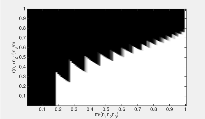
Second, we exam the phase transition phenomenon in tubal rank r and the number of measurements m. We set n1 = n2 = 30 and n3 = 5. We vary m between 1 and n1n2n3 where the tensor is completely discovered. For a fixed m, we generate all possible tubal ranks such that r(n1+n2-r)n3 ≤ m. For each (m, r) pair, we repeat the following procedure 10 times. We generate X0, A, y in the same way as the first experiment above. We declare X0 to be recovered if ‖ ˆX - X0‖F/‖X0‖F ≤ 10-3 . Figure 2 plots the fraction of correct recovery for each pair. The color of the cell in the figure reflects the empirical recovery rate of the 10 runs (scaled between 0 and 1). In all experiments, white denotes perfect recovery, while black denotes failure. It can be seen that there is a large region in which the recovery is correct. When the underlying tubal rank r of X0 is relatively larger, the required number of measurements for correct recovery is also larger. Such a result is consistent with our theoretical result. Similar phenomenon can be found in low-rank matrix recovery [Chandrasekaran et al., 2012].
6.2 Exact Tensor Completion
First, we verify the exact tensor completion guarantee in Theorem 6 on random data. We generate M ∈ Rn×n×n with tubal rank r byM = P∗Q, where the entries of P ∈ Rn×r×n and Q ∈ Rr×n×n are independently sampled from an N(0, 1/n) distribution. Then we sample m = pn3 elements uniformly fromMto form the known samples. A useful quantity for reference is the number of degrees of freedom dr = r(2n - r)n. The results in Table 1 shows that program (8) gives the correct recovery in the sense that the relative errors are small, less than 10-5 and the tubal ranks of the obtained solution are correct. These results well verify the recovery guarantee in Theorem 6.
Second, we examine the recovery phenomenon with varying tubal rank of M and varying sampling rate p. We consider two sizes of M ∈ Rn×n×n : (1) n = 40; (2) n = 50. We generate M = P ∗ Q, where the entries of P ∈ Rn×r×n and Q ∈ Rr×n×n are independently sampled from an N(0, 1/n) distribution. We set m = pn3 . We choose p in [0.01 : 0.01 : 0.99] and r = 1, 2, . . . , 30 in the case n = 40, and r = 1, 2, . . . , 35 in the case n = 50.
| n | r | m dr | p | rankt( ˆX) | ‖ ˆX-X‖F ‖X‖F |
|---|---|---|---|---|---|
| ∈ 50 | Rn×n×n 3 | = 4 | rankt(X0), 0.47 | = 3 | = r(2n 3.9e-7 |
| 50 | 5 | 3 | 0.57 | 5 | 3.5e-7 |
| 50 | 10 | 2 | 0.72 | 10 | 4.1e-7 |
| 100 | 5 | 4 | 0.39 | 5 | 1.4e-6 |
| 100 | 10 | 3 | 0.57 | 10 | 9.2e-7 |
| 100 | 15 | 2 | 0.56 | 15 | 8.4e-7 |
| 200 | 5 | 4 | 0.20 | 5 | 4.2e-6 |
| 200 | 10 | 3 | 0.29 | 10 | 3.2e-6 |
| 200 | 20 | 2 | 0.38 | 20 | 3.1e-6 |
| 300 | 10 | 4 | 0.26 | 10 | 5.1e-6 |
| 300 | 20 | 3 | 0.39 | 20 | 4.2e-6 |
| 300 | 30 | 3 | 0.57 | 30 | 2.9e-6 |
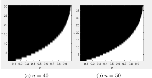
For each (r, p) triple, we simulate 10 test instances and declare a trial to be successful if the recovered ˆX satisfies ‖ ˆX -M‖F/‖M‖F ≤ 10-3 . Figure 3 plots the fraction of correct recovery for each triple (black = 0% and white = 100%). It can be seen that there is a large region in which the recovery is correct. Interestingly, the experiments reveal very similar plots for different n, suggesting that our asymptotic conditions for recovery may be conservative. Such a phenomenon is also consistent with the result in Theorem 6 which shows that the recovery is correct when the sampling rate p is not small and the tubal rank r is relatively low.
7 Conclusion
This paper first considers the exact guarantee of TNN minimization for low tubal rank tensor recovery from Gaussian measurements. We prove that TNN is a new instance of the atomic norm associated with certain atomic set. From the perspective of atomic norm minimization, we give the optimal estimation of the required measurements for the exact low tubal rank tensor recovery. Second, we give the exact recovery guarantee of TNN minimization for tensor completion. This result fixes the errors in the proofs of [Zhang and Aeron, 2017]. Numerical experiments verify our theoretical results.
By treating TNN as an instance of the atomic norm, we can get more results of low tubal rank recovery by using existing results, e.g., [Foygel and Mackey, 2014; Amelunxen et al., 2014]. Beyond the study on the convex TNN, it is also interesting to study the noncnovex models [Lu et al., 2015].
Acknowledgements
- Feng is partially supported by National University of Singapore startup grant R-263-000-C08-133 and Ministry of Education of Singapore AcRF Tier One grant R-263-000-C21112. Z. Lin was supported by National Basic Research Program of China (973 Program) (grant no. 2015CB352502), National Natural Science Foundation (NSF) of China (grant nos. 61625301 and 61731018), Qualcomm, and Microsoft Research Asia.
@inproceedings{ijcai2018p347,
  title     = {Exact Low Tubal Rank Tensor Recovery from Gaussian Measurements},
  author    = {Lu, Canyi and Feng, Jiashi and Lin, Zhouchen and Yan, Shuicheng},
  booktitle = {Proceedings of the Twenty-Seventh International Joint Conference on
               Artificial Intelligence, {IJCAI-18}},
  publisher = {International Joint Conferences on Artificial Intelligence Organization},
  editor    = {Jérôme Lang},
  pages     = {2504--2510},
  year      = {2018},
  month     = {7},
  note      = {Main track},
  doi       = {10.24963/ijcai.2018/347},
  url       = {https://doi.org/10.24963/ijcai.2018/347},
}
TY - CPAPER TI - Exact Low Tubal Rank Tensor Recovery from Gaussian Measurements AU - Lu, Canyi AU - Feng, Jiashi AU - Lin, Zhouchen AU - Yan, Shuicheng T2 - Proceedings of the Twenty-Seventh International Joint Conference on Artificial Intelligence, IJCAI-18 PB - International Joint Conferences on Artificial Intelligence Organization PY - 2018 SP - 2504 EP - 2510 DO - 10.24963/ijcai.2018/347 UR - https://doi.org/10.24963/ijcai.2018/347 ER -Copied
Machine-readable versions of this paper, for tools and AI agents:





