
Temporal Belief Memory: Imputing Missing Data during RNN Training
Proceedings of the Twenty-Seventh International Joint Conference on Artificial Intelligence. Main track. Pages 2326-2332.
https://doi.org/10.24963/ijcai.2018/322
Keywords
- Multidisciplinary Topics and Applications: Multidisciplinary Topics and Applications
- Machine Learning: Deep Learning
- Machine Learning Applications: Applications of Supervised Learning
- Machine Learning: Time-series;Data Streams
Abstract
We propose a bio-inspired approach named Temporal Belief Memory (TBM) for handling missing data with recurrent neural networks (RNNs). When modeling irregularly observed temporal sequences, conventional RNNs generally ignore the real-time intervals between consecutive observations. TBM is a missing value imputation method that considers the time continuity and captures latent missing patterns based on irregular real time intervals of the inputs. We evaluate our TBM approach with real-world electronic health records (EHRs) consisting of 52,919 visits and 4,224,567 events on a task of early prediction of septic shock. We compare TBM against multiple baselines including both domain experts' rules and the state-of-the-art missing data handling approach using both RNN and long-short term memory. The experimental results show that TBM outperforms all the competitive baseline approaches for the septic shock early prediction task.
- [Bengio and Gingras, 1995] Yoshua Bengio and Francois Gingras. Recurrent neural networks for missing or asyn- chronous data. In NIPS, pages 395-401, 1995.
- [Che et al., 2016] Zhengping Che, Sanjay Purushotham, Kyunghyun Cho, David Sontag, and Yan Liu. Recurrent neural networks for multivariate time series with missing values. CoRR, abs/1606.01865, 2016.
- [Cho et al., 2014] Kyunghyun Cho, Bart van Merrienboer, Caglar Gulcehre, Dzmitry Bahdanau, Fethi Bougares, Holger Schwenk, and Yoshua Bengio. Learning phrase representations using RNN encoder-decoder for statistical machine translation. In EMNLP, page 1724-1734, 2014.
- [Cismondi et al., 2013] Federico Cismondi, Andre Fialho, Susana Vieira, Shane Reti, João Sousa, and Stan Finkel- stein. Missing data in medical databases: Impute, delete or classify. AI in Medicine, 58(1), May 2013.
- [Cohen and Cohen, 1975] Jacob Cohen and Patricia Cohen. Applied Multiple Regression/Correlation Analysis for the Behavioral Sciences. John Wiley&Sons, New York, 1975.
- [Galimard et al., 2016] Jacques-Emmanuel Galimard, Sylvie Chevret, Camelia Protopopescu, and Matthieu Resche-Rigon. A multiple imputation approach for mnar mechanisms compatible with heckman's model. Statistics in medicine, 35, February 2016.
- [García-Laencina et al., 2015] Pedro García-Laencina, Pe- dro Abreu, Miguel Abreu, and Noémia Afonoso. Missing data imputation on the 5-year survival prediction of breast cancer patients with unknown discrete values. Computers in Biology and Medicine, 59(1), April 2015.
- [Gerstner and Kistler, 2002] Wulfram Gerstner and Werner Kistler. Spiking neuron models: single neurons, popula- tions, plasticity. Cambridge University Press, Cambridge, 2002.
- [Graves, 2013] Alex Graves. Generating sequences with re- current neural networks. CoRR, abs/1308.0850, 2013.
- [Ho et al., 2014] Joyce Ho, Cheng Lee, and Joydeep Ghosh. Septic shock prediction for patients with missing data. Management Information Systems, 5(1), April 2014.
- [Hochreiter and Schmidhuber, 1997] Sepp Hochreiter and Jurgen Schmidhuber. Long short-term memory. Neural Computation, 9(8), December 1997.
- [Hodgkin and Huxley, 1952] Alan Hodgkin and Andrew Huxley. A quantitative description of membrane current and its application to conduction and excitation in nerve. The Journal of Physiology, 117(4), August 1952.
- [Hsieh and Tang, 2013] Hung-Yi Hsieh and Kea-Tiong Tang. Hardware friendly probabilistic spiking neural network with long-term and short-term plasticity. Neural Networks and Learning Systems, 24(12), December 2013.
- [Kadri et al., 2017] Sameer Kadri, Chanu Rhee, Jeffrey Strich, Megan Morales, Samuel Hohmann, Jonathan Men- chaca, Anthony Suffredini, Robert Danner, and Michael Klompas. Estimating ten-year trends in septic shock in- cidence and mortality in united states academic medical centers using clinical data. Chest, 2017.
- [Kim et al., 2017] Han-Gyu Kim, Gil-Jin Jang, Ho-Jin Choi, Minho Kim, Young-Won Kim, and Jaehun Choi. Recur- rent neural networks with missing information imputation for medical examination data prediction. In BigComp, pages 317-323, February 2017.
- [Kingma and Ba, 2015] Diederik Kingma and Jimmy Ba. Adam: A method for stochastic optimization. In ICLR, 2015.
- [Kumar et al., 2006] Anand Kumar, Daniel Roberts, Ken- neth Wood, Bruce Light, Joseph Parrillo, Satendra Sharma, Robert Suppes, Daniel Feinstein, Sergio Zan- otti, Leo Taiberg, David Gurka, Aseem Kumar, and Mary Cheang. Duration of hypotension before initiation of ef- fective antimicrobial therapy is the critical determinant of survival in human septic shock. CCM, 34(6), June 2006.
- [Lipton et al., 2016] Zachary Lipton, David Kale, and Ran- dall Wetzel. Directly modeling missing data in sequences with RNNs: Improved classification of clinical time series. JMLR, 56, 2016.
- [Maass, 1997] Wolfgang Maass. Networks of spiking neu- rons: The third generation of neural network models. Neu- ral Networks, 10(9), 1997.
- [Neil et al., 2016] Daniel Neil, Michael Pfeiffer, and Shih- Chii Liu. Phased lstm: Accelerating recurrent network training for long or event-based sequences. In NIPS, 2016.
- [Parveen and Green, 2004] Shahla Parveen and Phil Green. Speech enhancement with missing data techniques using recurrent neural networks. In ICASSP, volume 1, pages I-733-736, May 2004.
- [Polat et al., 2017] Gizem Polat, Rustem Ugan, Elif Cadirci, and Zekai Halici. Sepsis and septic shock: Current treat- ment strategies and new approaches. EJM, 49, 2017.
- [Reinhart et al., 2017] Konrad Reinhart, Ron Daniels, Niran- jan Kissoon, Flavia Machado, Raymond Schachter, and Simon Finfer. Recognizaing sepsis as a global health priority-a who resolution. NEJM, August 2017.
- [Rubin and Little, 1987] Donald Rubin and Roderick Little. Statistical Analysis with Missing Data. John Wiley & Sons, Hoboken, NJ, 1987.
- [Singer et al., 2016] Mervyn Singer, Clifford Deutschman, Christopher Seymour, Manu Shankar-Hari, Djillali Annane, Michael Bauer, Rinaldo Bellomo, Gordon Bernard, Jean-Daniel Chiche, Craig Coopersmith, Richard Hotchkiss, Mitchell Levy, John Marshall, Greg Martin, Steven Opal, Gordon Rubenfeld, Tom van der Poll, Jean- Louis Vincent, and Derek Angus. The third international consensus definitions for sepsis and septic shock (sepsis- 3). AMA, 315(8), February 2016.
- [Tresp and Briegel, 1997] Volker Tresp and Thomas Briegel. A solution for missing data in recurrent neural networks with an application to blood glucose prediction. In NIPS, pages 971-977, 1997.
References were extracted automatically from the PDF and may contain errors.
Full text extracted automatically from the PDF; figures, tables and equations may differ. The PDF is the version of record.
1 Introduction
Multivariate time series data are ubiquitous in real-world dynamic systems such as health care and distributed sensor networks. In many of these systems, measurements are commonly acquired at irregular intervals. For example, many health care systems record large amounts of time series data in electronic health records (EHRs) for each patient's visit; during a patient's visit, the body temperatures are often measured a few times a day while the white blood cells are only measured every other day. As a result of merging such irregular data, real-world multivariate time series data is often plagued by missing values.
Generally speaking, the mechanisms of missing data can be divided into three categories: missing completely at random (MCAR), missing at random (MAR), and missing not at random (MNAR) [Rubin and Little, 1987]. In the domain of EHRs, for example, MCAR refers to missingness that is independent of all observed and unobserved values; one such example is when equipment failed to collect a patient's data. MAR refers to missingness that is independent of unobserved values but depends on the observed values: for example, patients with very good vital signs may not need to undergo certain lab tests. Finally, MNAR refers to missingness that depends on both observed values and unmeasured variables: for instance, a depressed patient might refuse a depression screening.
Ideally, different approaches should be applied depending on the missing mechanisms. For example, if the data is MCAR and the missing rate is low, we can delete the cases with missing values; if the missing rate is high, we might impute missing values with the mean. However, as many realworld datasets often have all three categories of missingness, various missing data approaches have been used, and some common approaches include forward-filling, hot-deck, EM imputation [Garc´ıa-Laencina et al., 2015], resampling [Cismondi et al., 2013], multiple imputation [Galimard et al., 2016] and so on. More recently, Lipton et al. showed using missing indicators (MI) [Rubin and Little, 1987] to be highly effective for handling temporal missing data [Lipton et al., 2016].
In this paper, we propose a bio-inspired imputation method, temporal belief memory (TBM), that considers the time continuity and captures latent missing patterns based on irregular real time intervals of inputs to handle missing data. More specifically, TBM computes a belief of the last observation over time for each feature and imputes a missing value based on that individual belief in both forward and backward directions. We evaluate the proposed TBM method and compare it with four competitive missing data handling methods - mean-substitution, forward-filling, expert knowledge based imputation rules - and the recent effective approach, missing indicator (MI) [Lipton et al., 2016]. These missing data handling methods are compared on two types of state-of-theart classifiers: RNNs and long short-term memory (LSTM) [Hochreiter and Schmidhuber, 1997]. Our empirical results showed TBM can effectively handle multivariate time series data with a high rate of missing values. It outperformed not only the two baseline methods (mean-substitution and forward-filling) but also the domain experts' rules and MI. TBM and MI tackle missing data from two different perspectives, since the best performance is obtained when we combine the two approaches.
Recurrent neural networks (RNNs), such as LSTM and gated recurrent unit (GRU) [Cho et al., 2014], have been shown to achieve the state-of-the-art results in many realword applications with multivariate time series data through deep hierarchical feature construction. Moreover, they can capture long-range dependencies in time series data in an effective manner. RNNs for missing data have been studied in earlier works [Bengio and Gingras, 1995], and applied for speech recognition and blood-glucose prediction [Parveen and Green, 2004; Tresp and Briegel, 1997]. Recently researchers tried to handle missingness in RNNs by concatenating missing entries, or incorporating a time based decay function, or synchronizing different sampling frequencies [Lipton et al., 2016; Che et al., 2016; Neil et al., 2016]. To our knowledge, however, no prior work has addressed the power of TBM, which can systematically model missing patterns in both forward and backward directions, with RNNs for sequence-labeling tasks.
Here, our task is early prediction of septic shock. Sepsis is a life-threatening organ dysfunction caused by a deregulated host response to infection [Singer et al., 2016]. As a leading cause of hospital death in the United States, sepsis affects nearly 30 million episodes and 6 million deaths per year worldwide [Reinhart et al., 2017]. From 2005 to 2014 Septic shock, the most severe complication of sepsis, incidence increased from 6.7 to 19.3 per 1,000 hospitalizations, while mortality decreased from 48.3% to 39.3% [Kadri et al., 2017]. Prior studies have indicated that early diagnosis and treatment of septic shock can prevent about 80% of sepsis deaths. On the contrary, over the first 6 hours after the onset of recurrent or persistent hypotension, every hour delay in antibiotic treatment leads to a 7.6% decrease in survival of septic patients [Kumar et al., 2006].
One major challenge associated with early prediction of sepsis/septic shock is its subtle but fast progression at early stages with lack of information. Sepsis has a wide range of potential symptoms, and its common indicators such as infection, fast heart rate, high/low body temperature, and low blood pressure [Polat et al., 2017] are highly likely to progress to other disease. Because of such delicate progressions, variables in the before-shock stage may either be measured infrequently or not measured at all. In result, the duration between two clinical events in EHRs can be long and the missing rate can be very high. For example, the EHRs used in this work were taken from large typical US hospitals, and on average more than 80% of data are missing and several variables' missing rates are above 99.9%. Thus, missing data handling can be a key factor in this early prediction task.
2 RelatedWork
2.1 The Hodgkin-HuxleyModel
Our TBM approach was originally inspired by a biological neural model proposed by [Hodgkin and Huxley, 1952], commonly referred to as the Hodgkin-Huxley model. The Hodgkin-Huxley model describes the electro-chemical information transmission of natural neurons with electrical circuits. It has been shown to realistically model biological neurons, and consistently inspired the advance of artificial neural networks, including deep learning.
Despite the great success of deep learning, the existing artificial neural networks still cannot match the human brain on many tasks. Therefore, some recent research on artificial neural networks returns to the biological roots of neurons and looks at how our brains function. Among them, spiking neural networks (SNNs) have gained increasing attention. SNNs can be seen as time dependent neural networks inspired by the Hodgkin-Huxley model and other bio-neuron models, and are often considered as the third generation of computational neural networks [Maass, 1997]. Compared with conventional artificial neural networks, SNNs take advantage of the precise timing of spikes generated by neurons and thus have greater computational power [Gerstner and Kistler, 2002]. Indeed, a probabilistic SNN outperformed deep networks for breast cancer prediction [Hsieh and Tang, 2013].
Although this work has a common ground with SNN in that the neural networks embrace a time concept to process inputs, we focus on the decaying mechanism on how bio-neurons handle missing signals, while most SNNs have concentrated on the spiking mechanism on how bio-neurons fire.
2.2 Missing Data Handling in RNNs
A recurrent neural network (RNN) is a type of deep neural network, designed to learn temporal patterns in sequential data. Although RNNs are theoretically able to find long-term dependencies underlying sequential data, classical RNNs often do not effectively capture them due to the vanishing and exploding gradient problem [Graves, 2013]. As variants of RNNs, LSTM [Hochreiter and Schmidhuber, 1997] and GRU [Cho et al., 2014] overcome these issues by incorporating multiple gating units into an RNN structure. A gating mechanism allows for explicit memory delete and update, and controls the flow of information in hidden units.
As frontier work for missing data handling for RNNs, [Bengio and Gingras, 1995] proposed an RNN structure for both missing inputs and asynchronous data that randomly initializes missing values and optimizes the filled values through backpropagation. In [Tresp and Briegel, 1997], they demonstrated a modified RNN for missing data handling, combined with a linear error model trained by an expectationmaximization technique. The experimental results show that their method improves performance in the glucose/insulin metabolism prediction task with respect to both conventional RNNs and various linear models.
Recently, [Lipton et al., 2016] showed the effectiveness of missing indicators (MI) with LSTM for the 128 phenotype prediction task using an EHR dataset. In their work, they gave an insight that LSTM is implicitly able to impute missing values based on its memory. About the same period, Phased LSTM [Neil et al., 2016] extends an LSTM unit by adding a time gate to align asynchronous streams, which allows the feature learning only when the time gate is open. On the other hand, [Kim et al., 2017] incorporated a forward-filling operation for missing data into RNN and LSTM, and tested it to a clinical variable prediction task. While all these proceeding approaches show their own achievements, TBM addresses the missing data problem in terms of an observation's reliable period based on the input timing.
Closely related to this work, GRU-D [Che et al., 2016] imputes missing values using a modified GRU, regulated by a temporal decay function with trainable weights. On a wide range of tasks, the authors showed that GRU-D often demonstrates performance comparable to MI. In their work, they introduce an input/ hidden state decay function, and impute missing values with the input decay and update the previous hidden state with the hidden state decay. Our TBM differs from GRU-D in terms of four aspects: 1) when an input is observed, GRU-D imputes missing values in a forward direction, while TBM bidirectionally updates the imputed values within a reliable time window; 2) GRU-D updates the hidden state with the trained decay rate, while TBM only uses errors backpropagated by RNN models to update its parameters and does not modify an RNN structure; 3) GRU-D's trainable parameters are weight matrices, while TBM's is time; finally, 4) MI [Lipton et al., 2016] is incorporated into GRU-D (the update/reset gates and the hidden state candidate), while in this work MI is not originally incorporated into TBM but they can be combined. In fact, we explored the effectiveness of MI only, TBM only and combining TBM and MI.
3 Methods
In this section, we describe how TBM is derived from the Hodgkin-Huxley model and how TBM's model parameters can be learned during RNN training.
3.1 Bio-inspiredMissing Data Handling
The Hodgkin-Huxley model explains how to propagate electro-chemical signals through bio-neurons, using the voltage equation defined as:
where t is the time interval between the current time and the last observed time, V is a voltage, v is the last voltage when the input ceases, I is an input current, R is resistance, and C is capacity. As shown in Equation (1), while input signals continuously come into the pre-synapse of neuron within a specific time interval (I > 0), the neuron accumulates the voltage into its membrane, and if the voltage goes beyond a threshold, the neuron fires and propagates the signal to other neurons. This process is explained by the accumulation function (Equation 1, Top). When the input signal stops to come into the pre-synapse (I = 0), the voltage gradually decreases over time, and if it goes below the threshold, the signal propagation stops, which is performed by the decay function (Equation 1, Bottom). It should be noted that the accumulating/decaying gradients of voltage depend on R ∗ C. As R∗C increases, the voltage changes less rapidly; as R∗C decreases, the voltage changes more rapidly.
For R ∗ C, there are two notable properties. First, when the signal ceases (I = 0), if the neuron has been already activated, the voltage is still valid at least within a specific time window. Second, since each neuron has its own resistance R and capacity C, each neuron has its own accumulating and decaying rate for voltage. That is, each neuron has its own time-based memory mechanism: how fast it accepts or forgets input signals.
Unlike continuous and frequent signals processed by bioneurons, real-world multivariate time series data such as EHRs are characterized by discrete and sparse data. Therefore, to apply the Hodgkin-Huxley model to our data, we need to reformulate the voltage equation. The accumulation function (Equation 1, Top) models bio-neurons' continuous behaviors toward input and thus better suits for high frequency data such as audio or video. The decay function (Equation 1, Bottom) is designed to model when there is no input, how the voltage V gradually decreases over time. Similarly, for EHRs, we can treat each observation as the initial voltage and model how our confidence on its value gradually decreases over time. Next, we describe how to combine this decay function mechanism with RNNs to address the data missingness.
3.2 Temporal Belief Memory
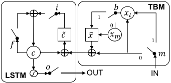
Figure 1 shows the architecture of a temporal belief memory (TBM), whose output connects to the input of LSTM. A TBM is a memory module that consists of two gating units (a missing gate m and a belief gate b), which collaboratively enables imputation of missing values based on beliefs of observations over time. The missing gate m indicates whether a value is missing (set to 1) or present (set to 0), and the belief gate b decides whether the last observation carries over to the imputed value ˜x based on the temporal reliability of the last observation. When an input is observed (m = 0), the observed value directly passes to the input of LSTM and updates the last observation, xl, with the current value. When an input is missing (m = 1), the belief gate b computes the belief of xl based on the time interval t between the current time and the last observed time. If the belief is greater than a threshold, it imputes the missing value with xl; otherwise, it sets the missing value to xm, which is the mean value of observations for each feature.
Once TBM imputes the missing values, LSTM is trained utilizing inputs with imputed values. The LSTM units are
where Wis a weight matrix, b is a bias, σ is a sigmoid activation function, tanh is a hyperbolic tangent function, and ⊙ denotes an element-wise vector product. In these equations, it, ft, and ot indicate the input, forget, and output gate at time t, while xt, ˜ ct, ct, and ht denote the input, memory cell state candidate, memory cell state, and memory cell output at time t, respectively. Although an LSTM is given as example in this section, TBM is scalable to variants of RNNs such as simple recurrent networks and GRUs.
Belief Gate
As described above, the decay function: V (t) = v∗e-t/(R∗C) (Equation 1, Bottom) can play a pivotal role to impute missing values. To reformulate it, we reinterpret a voltage V at time t as a temporal belief of an input value at current time t and then impute missing values based on the current belief.
First, we set the v in the decay function to be 1, which means whenever an input is observed, our belief on its value is 1; R ∗ C is combined into one parameter τ , which is conceptually a reliable-time-window variable that indicates how long we can trust the last observation when the current value is not observed. t is mapped to δt, the time interval between the last observation and the current time t. Thus we have a rather simple belief function at time t referred to as b′t :
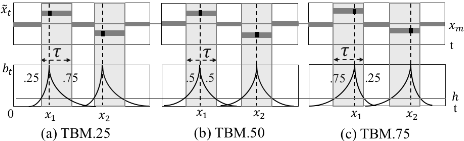
which models that the belief or the confidence of the last value gradually decreases over time. On the other hand, observations in EHRs are often reliable for a certain period in bidirectional ways. For example, if the current heart rate is 100, it is likely to be 100 a few minutes prior as well as a few minutes later. To incorporate the bidirectional nature of observations, we introduce a new parameter β into the equation above and result a new definition b′′ t:
where β is a hyper-parameter that controls a shift of the time window τ and the absolute value of δt is the time interval between the last observed time and the current time. Note that backward belief propagation can be implemented by mirroring the forward belief and the use of the absolute value of δt would support both the backward and forward cases. The lower part of Figure 2 shows the impact of different βs on the belief functions. Here based on different combinations, we have three settings of TBM: (a) TBM.25: 25% of backward and 75% of forward belief interval, (b) TBM.50: equal weights of backward and forward belief interval, and (c) TBM.75: 25% of backward and 75% of forward belief interval. Finally, we apply the unit step function with threshold h on b′′ t to get the belief gate, bt = θh(e(-β∗|δt|)/τ ) where if b′′ t in Equation 4 is greater than h, bt = 1; otherwise bt = 0.
Imputation
For a given time t, TBM imputes missing values using the missing gate mt and the belief gate bt. We denote an imputed value at time t with ˜xt, which is defined as
where xt is a current value, xl is a last value, and xm is a mean value for a feature. When a current value is observed (mt = 0), xt takes the current input xt, while when a current value is missing (mt = 1), xt takes the last value only if it is reliable (the output of belief gate is 1: bt = 1). Otherwise, it takes the mean value for the corresponding feature.
Note that by using the unit step function to transform b′′ t to bt, the imputed values will not converge to the mean value within the reliable-time-window, and the variance of the imputed ones will be close to the original values. By contrast, the mean substitution or b′′ t without the unit step function often abnormally creates average data points and decreases the variation of the imputed data. This decrease in individual variables is proportional to the number of missing data, and may considerably distort the correlations of variables when the missing rate is high [Cohen and Cohen, 1975].
4 Experiment
4.1 Data
Our dataset constitutes anonymized clinical multivariate time series data, extracted from the EHR system at Christiana Care Health System from July, 2013 to December, 2015. Each visit/episode consists of multiple temporal events such as medical readings and interventions. In total, there are 119,857 patients, 210,289 visits, and 10,412,729 medical events. Along with time stamps, identifiers, locations, and description, there are three categories of main attributes as follows:
- Vital signs: systolic blood pressure, mean arterial pressure, temperature, heart rate, respiratory rate, etc.
- Lab results: white blood cell count, Bands, BUN, procalcitonin, platelet, creatinine, bilirubin, C-reactive protein, lactate, sedimentation rate, etc.
- Intervention: oxygen source, change of oxygen source, FiO2, drug administration, intravenous therapy, etc.
Target Population and Labeling
The study population are patients with Suspected infection which was identified by the presence of any type of antibiotic, antiviral, or antifungal administration, or a positive test result of Point of Care Rapid, and it consists of 52,919 visits and 4,224,567 medical events. Note that the study population, the aforementioned rules for identifying suspected infection, and the septic shock labeling in next paragraph were determined by two leading clinicians with extensive experience on this subject from Mayo Clinic and Cristina Care Health System.
Supervised models depend heavily on the accurate label of the training dataset. However, acquiring the true label (i.e., septic shock and non septic shock) can be challenging. Although diagnosis codes, such as International Classification of Diseases, Ninth Revision (ICD-9), are widely used for clinical labeling, solely relying on ICD-9 can be problematic as it has been proven to have limited reliability due to the fact that its coding practice is used mainly for administrative and billing purpose. Indeed, it has been widely argued that ICD9 codes cannot be used for establishing reliable gold standards for various clinical conditions [Ho et al., 2014]. More importantly, ICD-9 cannot tell when septic shock occurs at event level, which is essential for our task. On the basis of the Third International Consensus Definitions for Sepsis and Septic Shock [Singer et al., 2016], our domain experts identified septic shock as having received vasopressor(s) or having had persistent hypotension (i.e., systolic blood pressure less than 90 mmHg or mean arterial pressure less than 65 mmHg for more than 1 hour) and enabled to diagnose septic shock at event level.
| Feature | Missing rate | Feature | Missing rate |
|---|---|---|---|
| Procalcitonin | 0.9998 | FiO2 | 0.8046 |
| CReactiveProtein | 0.9994 | MAP | 0.7735 |
| SedRate | 0.9992 | DistolicBP | 0.7214 |
| Bands | 0.9892 | SystolicBP | 0.7204 |
| BiliRubin | 0.9793 | PulseOx | 0.6369 |
| Lactate | 0.9723 | RespiratoryRate | 0.6261 |
| WBC | 0.9347 | HeartRate | 0.6064 |
| Platelet | 0.9341 | OxygenSource | 0.1267 |
| BUN | 0.9332 | ------- | --- |
| Creatinine | 0.9331 | Infection | 0.9438 |
| ChangeOxygenSrc. | 0.9137 | Inflammation | 0.6964 |
| Temperature | 0.8125 | OrganFailure | 0.7661 |
| Mean | 0.8184 |
When applying both ICD-9 and our clinical rules, we identified 1,869 shock positive visits and 23,901 negative visits. Given the imbalanced ratio of positive and negative shock visits, we further conducted a stratified random sampling on shock negative visits while keeping the same underlying distribution of age, gender, ethnicity, length of stay and the number of records in both positive and negative visits. As a result, the final dataset has 3,738 visits (1,869 positives and 1,869 negatives) and 145,421 events.
Missing Data Analysis
Each visit consists of irregular multivariate time series events with missing values and missing attributes, because different attributes are measured at different events. For example, vital signs are measured every 8 hours while lab values are measured only every 24 hours. Hence there may not be available readings for lab results when a new event is created for vital signs. Table 1 shows the missing rates of 23 features in our final dataset. On average, the missing rate is 81.84%.
Experiment Setup
To evaluate the proposed TBM framework, we conducted a series of experiments to test its effectiveness for early septic shock prediction using two types of classifiers: RNN and LSTM. For each classifier, we explored three TBM imputation modes: TBM.25, TBM.50, and TBM.75, described in Figure 2, and compared these against two widely used baseline methods: Mean and Forward, and the rules suggested by domain experts, Expert.
- Mean: fills all the missing values with the mean value for the corresponding feature, which is zero in our case since the data is standardized.
- Forward: fills the missing values with the last observation until the next value is observed.
- Expert: is defined by the domain experts; it fills the missing values with the last value within the fixed length of forward time window (8 hours for vital signs and 24 hours for lab tests), and fills the remaining ones with the mean value for the corresponding feature.
Additionally, our TBM modes are also compared against and with missing indicator (MI) given its effectiveness [Lipton et al., 2016]. When applying MI, we need to decide how to fill-in the missing values. In [Lipton et al., 2016], they used MI with zero-filling, forward-filling, and hand-engineeredfilling, respectively. In our comparison, we combined MI with Mean, Forward, and Expert, respectively. Also, we explored combining the three TBMs with MI to see whether combining them together would further improve our results.
To summarize, we used two classifiers: RNN and LSTM to compare the following twelve methods from four categories: the Base (Mean, Forward, Expert), the Base-MI (Mean+MI, Forward+MI, Expert+MI), the TBMs (TBM.25, TBM.50, TBM.75) and the TBMs combined with MI (TBM.25-MI, TBM.50-MI, TBM.75-MI). For both RNN and LSTM, we use one hidden layer with 30 hidden neurons and 32 maximum sequence length. We use the Adam optimizer [Kingma and Ba, 2015] with the batch size 30, and adopt early stopping with 7 patience after minimum 10 epochs.
Our evaluation metrics include accuracy, recall (sensitivity), precision (positive predictive value (PPV)), F1 score, and area under the ROC (receiver operator characteristic) curve (AUC). Accuracy, F1-score and AUC are widely used to measure the prediction performance for machine learning approaches. In the realm of medical science, researchers commonly refer to sensitivity (recall) and PPV for the annotation performance. Therefore, we include the metrics for both machine learning and medical science domains. In the learning process, we split data into 80% for training, 10% for validation, and 10% for test, and conduct 5-fold cross validation.
4.2 Results
Three-hour-before & overall shock prediction
Table 2 shows predictive performance results. The first column is the classifier, the second column is the missing data handling method, columns 3 to 7 present our evaluation metrics for the three-hour-before shock prediction, and the last column presents the AUC score for the overall shock prediction (i.e., 0-24 hour-before shock prediction).
For each classifier, Table 2 can be divided into four subsessions: Base, Base-MI, TBM, and TBM-MI. For each subsession, the best results are marked in bold. Also, for either classifier, the highest score per metric across all the models is underlined. Finally, the best model across all methods and two classifiers are labeled with ∗. In the following, we analyze predictive performance within each classifier and then compare across them.
For RNN classifier, Table 2 shows that for the three Base methods, the Expert outperforms the other two on all measures except for the precision. For the Base-MI methods: there is no clear winner but in general Mean-MI and Forward-MI split the lead. For TBM-based model, TBM.75 outperforms the other two on all measures except for the precision; finally, for the three TBM-MI methods, TBM.50-MI outperforms the other two except for the precision and overall. Across the four categories using RNN, the best performance (underlined) is generated using the TBM-based models. In general, based on the best results from each category, we have Base ≈ Base-MI < TBM-MI < TBM.
Next, for LSTM, Table 2 shows that for the three Base methods, the Expert outperforms the other two on all measures except for the precision and overall. For the BaseMI methods: Forward-MI outperforms the other two on all measures except for the recall and overall. For TBM-based model, TBM.75 outperforms the other two on all measures except for the precision; finally, for the three TBM-MI methods, TBM.75-MI outperforms the other two except for the recall. Across the four categories using LSTM, the best performance (underlined) is generated using the TBM-MI models. In general, based on the best results from each category, we have Base ≈ Base-MI<TBM<TBM-MI for LSTM.
Across all 12 methods and two base classifiers, the best results come from LSTM+TBM-MI. On both classifiers, the TBM models outperform not only the popular applied baselines and the domain experts' rules but also the state-of-theart approach MI. However, we assume that TBM and MI tackle missing data handling from two different perspectives so that our best performance is generated by combining the two approaches using LSTM.
Detailed analyses on early prediction
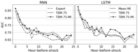
We also evaluate TBM's early prediction capacity comparing to other baseline methods based on the 0-24 hour-before shock prediction task. In particular, we compare the best TBM (TBM.75) to the best Base (Expert for RNN and MeanMI for LSTM) every hour between 0 to 10 hours and every two hours between 12 and 24 hours. Figure 3 (Left) shows that TBM.75 outperforms Expert throughout the time for RNN. Interestingly, when combining TBM with the previous state-of-the-art method, MI, TBM.75-MI does not outperform TBM.75. For LSTM (Figure 3, Right), TBM.75-MI outperforms Mean-MI except for the 12 hour-before shock prediction, while TBM.75 is comparable to MEAN-MI.
| Base | Method | 3 hour-before-shock | Overall | ||||
|---|---|---|---|---|---|---|---|
| classifier | Acc | Recall | Prec | F1 | AUC | AUC | |
| RNN | Mean | 0.7061 | 0.7076 | 0.7101 | 0.7077 | 0.7061 | 0.6875 |
| Forward | 0.7233 | 0.7264 | 0.7378 | 0.7270 | 0.7233 | 0.6968 | |
| Expert | 0.7367 | 0.7529 | 0.7113 | 0.7292 | 0.7368 | 0.6983 | |
| Mean-MI | 0.7306 | 0.7427 | 0.7102 | 0.7256 | 0.7306 | 0.6954 | |
| Forward-MI | 0.7306 | 0.7644 | 0.6792 | 0.7152 | 0.7308 | 0.6956 | |
| Expert-MI | 0.7100 | 0.7416 | 0.6726 | 0.6997 | 0.7102 | 0.6973 | |
| TBM.25 | 0.7567 | 0.7700 | 0.7368 | 0.7525 | 0.7568 | 0.7146 | |
| TBM.50 | 0.7511 | 0.7554 | 0.7522 | 0.7221 | 0.7511 | 0.7083 | |
| TBM.75 | 0.7628 | 0.7815 | 0.7357 | 0.7570 | 0.7630 | 0.7237 | |
| TBM.25-MI | 0.7467 | 0.7681 | 0.7168 | 0.7395 | 0.7469 | 0.7195 | |
| TBM.50-MI | 0.7556 | 0.7732 | 0.7312 | 0.7504 | 0.7557 | 0.7144 | |
| TBM.75-MI | 0.7528 | 0.7700 | 0.7313 | 0.7464 | 0.7530 | 0.7185 | |
| LSTM | Mean | 0.7078 | 0.7088 | 0.7102 | 0.7094 | 0.7078 | 0.6903 |
| Forward | 0.7156 | 0.7103 | 0.7423 | 0.7233 | 0.7154 | 0.6927 | |
| Expert | 0.7367 | 0.7429 | 0.7312 | 0.7358 | 0.7367 | 0.6918 | |
| Mean-MI | 0.7267 | 0.7346 | 0.7300 | 0.7276 | 0.7266 | 0.7107 | |
| Forward-MI | 0.7300 | 0.7263 | 0.7644 | 0.7395 | 0.7299 | 0.7067 | |
| Expert-MI | 0.7217 | 0.7174 | 0.7378 | 0.7249 | 0.7215 | 0.7058 | |
| TBM.25 | 0.7556 | 0.7573 | 0.7589 | 0.7569 | 0.7556 | 0.7188 | |
| TBM.50 | 0.7606 | 0.7725 | 0.7457 | 0.7576 | 0.7607 | 0.7184 | |
| TBM.75 | 0.7633 | 0.7751 | 0.7456 | 0.7593 | 0.7635 | 0.7245 | |
| TBM.25-MI | 0.7739 | 0.8085* | 0.7246 | 0.7623 | 0.7742 | 0.7262 | |
| TBM.50-MI | 0.7683 | 0.8002 | 0.7213 | 0.7572 | 0.7686 | 0.7322 | |
| TBM.75-MI | 0.7839* | 0.7900 | 0.7777* | 0.7832* | 0.7840* | 0.7340* | |
5 Conclusion
Missing data pervading in real-world multivariate time series datasets pose significant challenges in deriving robust predictive models for these real-world applications. More challengingly, the categories of missing data in these datasets are mingled or difficult to identify. To address this challenge, we have investigated missing data handling methods with RNNs and LSTMs, and examined early prediction of septic shock using imputed missing values in EHR. We have introduced a bidirectional time-based imputation method, called TBM, which was inspired by bio-neurons' behaviors. Empirical evaluations demonstrate that TBM achieves the best performance in the septic shock early prediction task, outperforming four competitive missing data handling methods.
Rather than use the pre-defined βs like in this study, in the future, we will further optimize TBMwith respect to the model hyperparameter β, which adjusts the bidirectional portions of reliable-time-window. Another interesting line of research is to investigate the interpretation of the reliable-timewindow τ , which can suggest a desirable sampling frequency for each feature to clinical and medical experts. Finally, it will be important to evaluate robustness and generalizability of TBM by investigating the septic shock early prediction framework for other EHR datasets such as MIMIC-III and as well as other disease prediction tasks or different prediction tasks on multivariate time-series data suffering a high rate of missing values in other domains.
Acknowledgements
This research is supported by the NSF Grants #1522107 and #1651909.
@inproceedings{ijcai2018p322,
  title     = {Temporal Belief Memory: Imputing Missing Data during RNN Training},
  author    = {Kim, Yeo Jin and Chi, Min},
  booktitle = {Proceedings of the Twenty-Seventh International Joint Conference on
               Artificial Intelligence, {IJCAI-18}},
  publisher = {International Joint Conferences on Artificial Intelligence Organization},
  editor    = {Jérôme Lang},
  pages     = {2326--2332},
  year      = {2018},
  month     = {7},
  note      = {Main track},
  doi       = {10.24963/ijcai.2018/322},
  url       = {https://doi.org/10.24963/ijcai.2018/322},
}
TY - CPAPER TI - Temporal Belief Memory: Imputing Missing Data during RNN Training AU - Kim, Yeo Jin AU - Chi, Min T2 - Proceedings of the Twenty-Seventh International Joint Conference on Artificial Intelligence, IJCAI-18 PB - International Joint Conferences on Artificial Intelligence Organization PY - 2018 SP - 2326 EP - 2332 DO - 10.24963/ijcai.2018/322 UR - https://doi.org/10.24963/ijcai.2018/322 ER -Copied
Machine-readable versions of this paper, for tools and AI agents:





