
Efficient DNN Neuron Pruning by Minimizing Layer-wise Nonlinear Reconstruction Error
Proceedings of the Twenty-Seventh International Joint Conference on Artificial Intelligence. Main track. Pages 2298-2304.
https://doi.org/10.24963/ijcai.2018/318
© 2018 International Joint Conferences on Artificial Intelligence
Keywords
- Machine Learning: Feature Selection ; Learning Sparse Models
- Machine Learning: Neural Networks
- Machine Learning Applications: Applications of Supervised Learning
- Machine Learning: Deep Learning
Abstract
Deep neural networks (DNNs) have achieved great success, but the applications to mobile devices are limited due to their huge model size and low inference speed. Much effort thus has been devoted to pruning DNNs. Layer-wise neuron pruning methods have shown their effectiveness, which minimize the reconstruction error of linear response with a limited number of neurons in each single layer pruning. In this paper, we propose a new layer-wise neuron pruning approach by minimizing the reconstruction error of nonlinear units, which might be more reasonable since the error before and after activation can change significantly. An iterative optimization procedure combining greedy selection with gradient decent is proposed for single layer pruning. Experimental results on benchmark DNN models show the superiority of the proposed approach. Particularly, for VGGNet, the proposed approach can compress its disk space by 13.6× and bring a speedup of 3.7×; for AlexNet, it can achieve a compression rate of 4.1× and a speedup of 2.2×, respectively.
- [Alvarez and Salzmann, 2016] J. M. Alvarez and M. Salz- mann. Learning the number of neurons in deep networks. In Advances in Neural Information Processing Systems 29 (NIPS'16), pages 2270-2278, Barcelona, Spain, 2016.
- [Courbariaux et al., 2016] M. Courbariaux, I. Hubara, D. Soudry, R. El-Yaniv, and Y. Bengio. Binarized neural networks: Training deep neural networks with weights and activations constrained to + 1 or -1. arXiv preprint arXiv:1602.02830, 2016.
- [Dong et al., 2017] X. Dong, S.-Y. Chen, and S. Pan. Learn- ing to prune deep neural networks via layer-wise optimal brain surgeon. In Advances in Neural Information Pro- cessing Systems 30 (NIPS'17), pages 4860-4874, Long Beach, CA, 2017.
- [Guo et al., 2016] Y.-W. Guo, A.-B. Yao, and Y.-R. Chen. Dynamic network surgery for efficient dnns. In Advances In Neural Information Processing Systems 29 (NIPS'16), pages 1379-1387, Barcelona, Spain, 2016.
- [Han et al., 2015] S. Han, J. Pool, J. Tran, and W. Dally. Learning both weights and connections for efficient neu- ral network. In Advances in Neural Information Process- ing Systems 28 (NIPS'15), pages 1135-1143, Montreal, Canada, 2015.
- [He et al., 2017] Y.-H. He, X.-Y. Zhang, and J. Sun. Chan- nel pruning for accelerating very deep neural networks. In Proceedings of the 16th IEEE International Conference on Computer Vision (ICCV'17), pages 1398-1406, Venice, Italy, 2017.
- [Ioffe and Szegedy, 2015] S. Ioffe and C. Szegedy. Batch normalization: Accelerating deep network training by reducing internal covariate shift. In Proceedings of the 32nd International Conference on Machine Learning (ICML'15), pages 448-456, Lille, France, 2015.
- [Jaderberg et al., 2014] M. Jaderberg, A. Vedaldi, and A. Zisserman. Speeding up convolutional neural net- works with low rank expansions. arXiv preprint arXiv:1405.3866, 2014.
- [Jia et al., 2014] Y.-Q. Jia, E. Shelhamer, J. Donahue, S. Karayev, J. Long, R. B. Girshick, S. Guadarrama, and T. Darrell. Caffe: Convolutional architecture for fast fea- ture embedding. In Proceedings of the 22nd ACM inter- national conference on Multimedia (MM'14), pages 675- 678, Orlando, FL, 2014.
- [Krizhevsky and Hinton, 2009] A. Krizhevsky and G. Hin- ton. Learning multiple layers of features from tiny images. 2009.
- [LeCun et al., 1998] Y. LeCun, L. Bottou, Y. Bengio, and P. Haffner. Gradient-based learning applied to document recognition. Proceedings of the IEEE, 86(11):2278-2324, 1998.
- [Li et al., 2016] H. Li, A. Kadav, I. Durdanovic, H. Samet, and H. P. Graf. Pruning filters for efficient convnets. arXiv preprint arXiv:1608.08710, 2016.
- [Liu et al., 2017] Z. Liu, J.-G. Li, Z.-Q. Shen, G. Huang, S.- M. Yan, and C.-S. Zhang. Learning efficient convolutional networks through network slimming. In Proceedings of the 16th IEEE International Conference on Computer Vision (ICCV'17), pages 2755-2763, Venice, Italy, 2017.
- [Luo et al., 2017] J.-H. Luo, J.-X. Wu, and W.-Y. Lin. Thinet: A filter level pruning method for deep neural net- work compression. In Proceedings of the 16th IEEE In- ternational Conference on Computer Vision (ICCV'17), pages 5068-5076, Venice, Italy, 2017.
- [Nair and Hinton, 2010] V. Nair and G. E. Hinton. Rectified linear units improve restricted boltzmann machines. In Proceedings of the 27th International Conference on Ma- chine Learning (ICML'10), pages 807-814, Haifa, Israel, 2010.
- [Russakovsky et al., 2015] O. Russakovsky, J. Deng, H. Su, J. Krause, S. Satheesh, S. Ma, Z.-H. Huang, A. Karpathy, A. Khosla, M. S. Bernstein, A. C. Berg, and F.-F. Li. Im- agenet large scale visual recognition challenge. Interna- tional Journal of Computer Vision, 115(3):211-252, 2015.
- [Wen et al., 2016] W. Wen, C.-P. Wu, Y.-D. Wang, Y.-R. Chen, and H. Li. Learning structured sparsity in deep neu- ral networks. In Advances in Neural Information Process- ing Systems 29 (NIPS'16), pages 2074-2082, Barcelona, Spain, 2016.
- [Zhang et al., 2015] X.-Y. Zhang, J.-H. Zou, X. Ming, K.- M. He, and J. Sun. Efficient and accurate approximations of nonlinear convolutional networks. In Proceedings of the 28th IEEE Conference on Computer Vision and Pattern Recognition (CVPR'15), pages 1984-1992, Boston, MA, 2015.
References were extracted automatically from the PDF and may contain errors.
Full text extracted automatically from the PDF; figures, tables and equations may differ. The PDF is the version of record.
1 Introduction
In recent years, deep neural networks (DNNs) have made great success in many areas. However, DNNs usually have large storage overhead and low inference speed, which hinder their application to resource-limited devices, e.g., mobile phones. Many methods thus have been proposed to compress and accelerate DNN models, such as tensor decomposition [Jaderberg et al., 2014; Zhang et al., 2015], weight quantization [Courbariaux et al., 2016], weight pruning [Han et al., 2015; Guo et al., 2016; Dong et al., 2017] and neuron pruning [Wen et al., 2016; Alvarez and Salzmann, 2016; Li et al., 2016; Liu et al., 2017; He et al., 2017; Luo et al., 2017]. The proposed method falls into the class of neuron pruning.
∗This work was supported in part by the National Key Research and Development Program of China (2017YFB1003102), the NSFC (61672478), the Science and Technology Innovation Committee Foundation of Shenzhen (ZDSYS201703031748284), and the Royal Society Newton Advanced Fellowship (NA150123).
Different from weight pruning, which produces irregular sparsity by setting unimportant weights to zeros, neuron pruning directly removes redundant neurons (or channels for CNN) and produces a more compact structure. The advantages of neuron pruning mainly include: a) both disk usage and runtime memory are reduced; b) the pruned model can be accelerated without the need of extra sparse matrix library or custom hardware; c) neuron pruning can be combined with other techniques like tensor decomposition or weight quantization to further reduce computational cost [He et al., 2017].
Existing neuron pruning methods usually first prune neurons according to some criterion, and then retrain the pruned model by minimizing some loss function. They can be divided into two classes according to the difference of the employed loss function. The first class considers the loss of the entire model, and thus directly prunes all the neurons. For example, Li et al. [2016] first prune neurons with small absolute sum of incoming weights and then fine-tune the pruned model to regain accuracy. Some works combine the pruning and the retraining into one framework by adding regularization terms (which penalize unimportant neurons) to the loss function, such as group lasso in [Wen et al., 2016; Alvarez and Salzmann, 2016] and L1 regularization of batch normalization scaling factor in network slimming [Liu et al., 2017]. The second class considers the layer-wise loss and thus prunes neurons layer by layer. Previous works are mainly to minimize layer-wise linear reconstruction error (LRE), which is the Euclidean distance between linear activation (namely values before nonlinear activation functions) of the unpruned model and that of the pruned model. For example, in the pruning of each layer, He et al. [2017] use lasso regression to choose informative neurons and Luo et al. [2017] use a simple greedy step to select important neurons; then both methods use the ordinary least squares approach to minimize LRE.
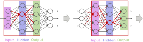
Layer-wise pruning has been shown more efficient than pruning all the neurons directly [He et al., 2017; Luo et al., 2017]. LRE considers the Euclidean distance in the input space of nonlinear activation functions, which, however, does not truly reflect the distance in the output space well. Taking the widely used activation function ReLU [Nair and Hinton, 2010] r(x) = max(0, x) as an example, the Euclidean distance can be large between two negative input values, but would become 0 after activation. Thus, nonlinear reconstruction error (NRE), which computes the Euclidean distance between nonlinear activation values of the unpruned model and those of the pruned model, can be a more reasonable metric than LRE when performing layer-wise pruning.
In this paper, we propose to optimize NRE in layer-wise neuron pruning. Specifically, we extract a corresponding 3layer subnetwork when pruning each single layer as shown in Figure 1. In this subnetwork, we adopt an iterative procedure to prune neurons of the hidden layer and minimize NRE of the output layer. Within each iteration, a greedy selection algorithm is employed to prune unimportant neurons and a modified gradient descent is used to minimize NRE. Empirical results on several DNN benchmark models show that the proposed method can prune more neurons than several state-of-the-art neuron pruning methods under the almost same level of accuracy drop.
The rest of the paper is organized as follows. Section 2 presents the proposed approach. In Section 3, we conduct experiments. Section 4 finally concludes the paper.
2 The Proposed Approach
In this section, we first present the whole framework of the proposed approach, then formulate the NRE objective function and present our method to prune one single layer, and finally discuss the hyperparameter tuning. Note that although we demonstrate our approach with fully-connected neural networks, it can be easily generalized to other types of DNNs.
2.1 Framework
We summarize our neuron pruning method in Algorithm 1. The core of the algorithm consists of two nested loops. The outer loop is designed to prune a pre-trained DNN model from bottom layer to top layer. The inner loop concentrates on single layer pruning. We solve single layer pruning by modeling a 3-layer subnetwork. Such modeling enables us to directly utilize off-the-shelf deep learning frameworks as well as GPUs.
Fine-tuning is helpful to regain the original accuracy. In order to save time, we do not use fine-tuning after single layer pruning but only fine-tune the model after pruning all layers.
Although sharing the similar framework, there are two major differences between the proposed method and previous layer-wise pruning methods [He et al., 2017; Luo et al., 2017]: 1) we propose to minimize layer-wise NRE, which is more reasonable than previously used LRE; 2) to prune neurons of one layer, we present an iterative algorithm and each iteration includes neuron selection and weights optimization, which is significantly different from previously used optimization methods.
2.2 Formulation
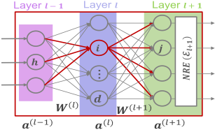
In this subsection, we introduce the formulation of optimizing NRE with a limited number of neurons in one single layer pruning. A DNN model with L layers is represented as {W (l) : 1 ≤ l ≤ L}, where W (l) denotes the weight matrix of layer l. We use a(l) to denote nonlinear response in layer l, and m(l) to denote a binary mask in which its entries indicate whether a neuron is pruned (value 0) or not (value 1), thus a pruned model can be represented as {W (l) ,m(l) : 1 ≤ l ≤ L}. Suppose that there are d neurons in layer l, then we have a(l) ,m(l) ∈ Rd . We also use W (l) i to denote the ith row or the ith column in W (l) , which actually indicates incoming weights or outgoing weights of a neuron. The connection between neuron i in layer l and neuron h in layer l-1 is denoted as W (l) ih . The notations are illustrated in Figure 2.
For pruning layer l, a 3-layer subnetwork {W (l) ,W (l+1) } is extracted. When pruning neurons in layer l, W (l) and W (l+1) are optimized by minimizing NRE of layer l + 1, which in fact is the Euclidean distance between two nonlinear outputs:
where o(l+1) denotes the nonlinear output of layer l +1 from the pre-trained model, N is the number of neurons in layer l + 1, λ is a scaling factor and ‖ · ‖2 denotes ℓ2-norm. Note that a(l+1) is calculated from W (l+1) and a(l) , and neuron pruning in layer l can be represented by the mask vector m(l) .
Thus, the optimization problem can be formulated as:
where a(l) = r(W (l) (a(l-1) ⊙m(l-1) )), r(·) is a nonlinear activation function, kl is the constraint on neuron numbers in layer l, ⊙ means element-wise multiplication and ‖ · ‖0 denotes the number of nonzeros.
2.3 Optimization
Due to the cardinality constraint kl and the nonlinear function r(·), Eq. (2) is generally NP-hard, thus we adopt an iterative greedy selection procedure to optimize Eq. (2). Within each iteration, the most important kl neurons are first selected to satisfy the cardinality constraint, after which a modified gradient descent step is used to minimize the NRE. These two steps are alternatively taken until convergence or halting conditions are satisfied.
Greedy Selection
To measure the importance of neurons, we first analyze the sensitivity of NRE with respect to each neuron. Unlike previous works [Li et al., 2016; He et al., 2017] that only consider a neuron's incoming or outgoing weights, we take both into consideration. Concretely, the sensitivity of neuron i in layer l is computed as:
which indicates the influence to the next layer if pruning neuron i. Note that a(l) i is calculated from a(l-1) and W (l) i , in which a(l-1) is data-dependent, thus the exact calculation of a(l) i needs to traverse the entire dataset and is timeconsuming. Inspired by [Li et al., 2016], we adopt a heuristic rule that a(l) i can be approximately determined by its incoming weights, namely ∑h (W (l) ih )2 . Therefore, the computation of δ(l) i is updated as:
which is the quadratic sum of incoming weights multiplying the quadratic sum of outgoing weights of neuron i. After computing each neuron's sensitivity, neurons with the kl largest sensitivity values are selected. We denote the kl-th largest value in δ(l) as δkl , then the mask m(l) can be updated by:
Gradient Descent
Given the binary mask m(l) , perhaps the easiest way of pruning neurons is to replace a(l) by a(l) ⊙m(l) in forward propagation. This will make weights connected to pruned neurons keep unchanged, thus cause pruned neurons always to
Algorithm 1 The Proposed Approach
Input: {̂ W (l) , kl : 1 ≤ l ≤ L}: the pre-trained model and the cardinality constraints on the neurons of each layer.
Output: {W (l) ,m(l) : 1 ≤ l ≤ L}: weights and neuron masks of the pruned model
- 1: Initialize: W (l) ← ̂ W (l) , m(l) ← 1, for ∀1 ≤ l ≤ L
- 2: for l = 1 to L-1 do
- 3: Extract a 3-layer subnetwork {W (l) ,W (l+1) } from the pruned model
- 4: repeat
- 5: Compute sensitivities of neurons by Eq. (4)
- 6: Updatem(l) by Eq. (5) with ‖m(l) ‖0 = kl
- 7: Forward propagation and compute El+1 by Eq. (7)
- 8: UpdateW (l+1) ,W (l) by Eqs. (8) and (9)
- 9: iter ← iter + 1
- 10: until converged or iter = itermax
- 11: end for
- 12: Fine-tuning
be pruned in the following iterations, since the remaining weights will probably get larger which results in even larger sensitivities of the unpruned neurons.
However, it is possible that the above greedy selection step selects wrong neurons or some selected neurons become unimportant after a few iterations. So it is desirable to maintain a dynamic network structure by making the pruned neurons have chance to come back according to their changing sensitivities. Inspired by [Guo et al., 2016], which made efficient weight pruning by incorporating weight splicing, we modify standard gradient descent as follows:
1) Forward and Backward Propagation. In these two steps, a masked version of W (l+1) is used, that is defined as:
which in fact sets weights connected to pruned neurons to zeros. It should be noticed that the unmaskedW (l+1) is also preserved to be used in the gradient update step. Thus, the NRE in layer l + 1 is computed as:
In fact, using masked W (l+1) has the same effect as using a(l) ⊙m(l) , since both of them perform neuron pruning in forward propagation. However, with masked W (l+1) , the pruned neurons have non-zero activation values in a(l) . Thus, their weights in masked W (l+1) have non-zero gradients, although being zeros themselves.
2) Gradient Update. In this step, an unmasked version of W (l+1) is used and updated by:
where η is the learning rate. Note that W (l) is also updated by a gradient descent step:
After updatingW (l+1) andW (l) , this iteration is finished. In the next iteration, the sensitivity of neurons will be recalculated and their masks will be updated.
2.4 Hyperparameter Tuning
The cardinality constraint kl plays an important role in single layer pruning. Instead of performing exhaustive search, kl is determined by employing a similar strategy as in [Han et al., 2015]. First, neurons are sorted by their sensitivities, and then a trade-off curve is plotted between the accuracy and the number of pruned neurons. After that, the value of kl is empirically determined when the curve begins to drop quickly.
The scaling factor λ is adopted to rescale the NRE to a desirable range, so that the gradients do not explode or become too small to minimize NRE efficiently. In order to avoid introducing extra layer-wise parameters, we use a uniform scaling factor across all layers of a model.
3 Experiment
In this section, the proposed approach is empirically evaluated on three benchmark data sets: MNIST [LeCun et al., 1998], CIFAR-10 [Krizhevsky and Hinton, 2009] and ILSVRC2012 [Russakovsky et al., 2015]. We compare it with four state-of-the-art neuron pruning methods, i.e., Weight Sum [Li et al., 2016], Group Lasso [Wen et al., 2016], Network Slimming [Liu et al., 2017] and ThiNet [Luo et al., 2017]. Note that ThiNet is also a layerwise pruning method as ours. The proposed approach is implemented with the Caffe framework [Jia et al., 2014].
3.1 Experimental Setup
Datasets and DNN Models
For MNIST, a 4-layer MLP with neurons 784-500-300-10 is used as in [Wen et al., 2016]. For CIFAR-10, we use a VGGNet variant [Li et al., 2016] which has 13 convolutional layers. ILSVRC2012 is a subset of the huge ImageNet data set and contains over 1.2 million images. For ILSVRC2012, we use AlexNet with batch normalization [Ioffe and Szegedy, 2015] which has 5 convolutional layers and 3 fully-connected layers. We train these DNNs from scratch as the baseline models. The MLP baseline is trained with 18,000 iterations and an initial learning rate of 0.1 which is multiplied by 0.1 after 1/3 and 2/3 fraction of training iterations. The VGGNet baseline is trained with 64,000 iterations, and also with an initial learning rate of 0.1 which is multiplied by 0.1 after 1/2 and 3/4 fraction of training iterations. The AlexNet baseline is trained using the standard protocol in Caffe. All the baseline training uses a batchsize of 128, a momentum of 0.9 and a weight decay of 0.0005.
Implementation Details
The proposed pruning method computes NRE on 5,000 images randomly selected from the training data set as in [He et al., 2017]. For single layer pruning, the proposed method uses 1,500, 400 and 3,000 iterations to minimize NRE for MLP, VGGNet and AlexNet, respectively. The number of iterations only takes 1/12, 1/160 and 1/300 of the original baseline training, respectively. The scaling factor λ takes 512 for all the three DNN models. The neuron masks will not be updated in the second half iterations to get a more stable performance. Fine-tuning is also used to regain accuracy. We fine-tune the pruned MLP, VGGNet, AlexNet with an initial learning rate of 0.1, 0.01, 0.001 and with 12,000, 32,000, 45,000 iterations, respectively. For fine-tuning, the batchsize, momentum, weight decay and learning rate decay policy are the same as baseline training. Experiments are conducted on NVIDIA TITAN X (Pascal) graphics card. The speedup is measured on a single-thread Intel Xeon E5-2683 CPU.
Evaluation Metrics
For MNIST and CIFAR-10, the accuracy on the test set is reported. For ILSVRC2012, the top-1 accuracy on center 224×224 crop of the validation set is reported. We also report the actual compression rate and speedup, where the former is defined as the disk usage of the unpruned model divided by that of the pruned model, and the latter is defined as actual inference time of the unpruned model divided by that of the pruned model. Note that the results of the proposed method are averaged over 5 independent runs to reduce randomness, except for AlexNet due to time limit.
3.2 Overall Comparison Results
First of all, we report the performance of the proposed method and four compared methods after pruning and fine-tuning all layers of a model. The overall comparison results on three DNN models are shown in Table 1. Note that all methods use the same fine-tuning strategy for fair comparison.
For MLP, it can be observed that the proposed method achieves the best performance in all evaluation metrics. It can prune the neurons of MLP's two hidden layers from (500, 300) to (90, 40), which results in a compression rate of 7.0× and a speedup of 4.3×. Under the same accuracy drop, the proposed method can prune more neurons and reduce more computational cost than other methods. Note that the computational cost is measured by the ratio of pruned float point operations (FLOPs), which is equal to the ratio of pruned parameters for fully-connected DNNs because both of them are directly determined by the dimension of weight matrix.
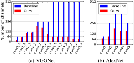
For VGGNet, the proposed method can compress its disk usage by 13.6× (from 57MB to 4.2MB) and reach a speedup of 3.7×, both of which are better than the compared methods, although the accuracy of Network Slimming is slightly better than ours. The layer-wise comparison of the number of channels between the baseline model and our pruned model can be found in Figure 3(a). We can see that the proposed method can prune much more neurons in layers from conv3 3 to conv5 3 than in other layers, which indicates that the last several layers of VGGNet are more redundant. Note that in addition to the proposed method, ThiNet also performs well, which verifies the effectiveness of layer-wise neuron pruning schemes.
| Models | Methods | Acc (%) | Parameters pruned | (%) FLOPs pruned | (%) Disk usage | Comp. rate | Speedup |
|---|---|---|---|---|---|---|---|
| MLP (on MNIST) | Baseline | 98.6 | 0.0 | 0.0 | 2.1MB | 1.0 | 1.0 |
| Weight Sum | 98.5 | 79.5 | 79.5 | 0.44MB | 4.8 | 2.9 | |
| Group Lasso† | 98.5 | 83.5 | 83.5 | - | - | - | |
| Network Slimming∗ | 98.5 | 84.4 | 84.4 | 0.34MB | 6.2 | 4.1 | |
| ThiNet | 98.5 | 80.8 | 80.8 | 0.41MB | 5.1 | 3.9 | |
| Ours | 98.5 | 86.3 | 86.3 | 0.30MB | 7.0 | 4.3 | |
| VGGNet CIFAR-10) | Baseline | 93.46 | 0.0 | 0.0 | 57MB | 1.0 | 1.0 |
| Weight Sum‡ | 93.40 | 64.0 | 34.2 | 21MB | 2.7 | 1.8 | |
| Group Lasso | 93.41 | 88.8 | 52.3 | 6.4MB | 8.9 | 2.8 | |
| (on | Network Slimming∗ | 93.80 | 88.5 | 51.0 | - | 8.7 | - |
| ThiNet | 93.41 | 91.9 | 60.6 | 4.6MB | 12.4 | 3.1 | |
| Ours | 93.40 | 92.7 | 67.6 | 4.2MB | 13.6 | 3.7 | |
| AlexNet ILSVRC2012) | Baseline | 58.30 | 0.0 | 0.0 | 239MB | 1.0 | 1.0 |
| Weight Sum | 54.99 | 73.3 | 43.8 | 64MB | 3.7 | 1.6 | |
| Group Lasso | 54.31 | 67.4 | 51.4 | 78MB | 3.1 | 1.8 | |
| (on | Network Slimming | 53.87 | 70.5 | 46.9 | 71MB | 3.4 | 1.7 |
| ThiNet | 53.67 | 75.6 | 55.9 | 59MB | 4.1 | 1.9 | |
| Ours | 54.63 | 76.1 | 63.7 | 58MB | 4.1 | 2.2 |
Regarding AlexNet, similar with previous results, the proposed method can prune more parameters and FLOPs than the compared methods under the same level of accuracy drop. Concretely, our approach can compress its disk space from 239MB to 58MB, which mainly results from pruning the neurons of two fully-connected layers from (4096, 4096) to (1280, 2000) because the fully-connected layers take the most part (∼96%) of overall parameters for AlexNet. The proposed method can also accelerate the inference time of AlexNet by 2.2×, which mainly comes from pruning the channels of convolutional layers (Figure 3(b)) because the convolutional layers account for a great proportion (∼93%) of overall FLOPs. Note that although ThiNet has comparable compression rate as ours, its accuracy is much worse.
3.3 Analysis of the Proposed Approach
Note that we prune a DNN model in a layer-wise manner by minimizing NRE, thus in this subsection we analyze the proposed approach in the following aspects: the effectiveness of single layer pruning, the convergence of the proposed method and the validity of using NRE as the optimization objective.

Single Layer Pruning
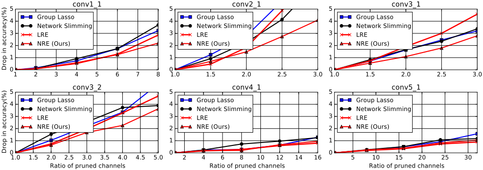
Recall that we adopt an iterative algorithm to minimize NRE within a 3-layer subnetwork when performing single layer pruning. It should be noticed that given a 3-layer subnetwork, there are also other methods which can minimize NRE, such as Group Lasso and Network Slimming, thus we compare the proposed method with these two approaches. To demonstrate the effectiveness of NRE, we also compare with a variant of the proposed method in which NRE is replaced with LRE, and we call it LRE for simplicity. Note that only neurons of one layer are pruned and the other layers remain the same as baseline model. All methods use the same number of iterations (400), the same learning rate (0.01) and no fine-tuning is used. We measure the accuracy drop of different methods by varying the ratio of pruned channels which is defined as the total number of channels in this layer divided by the number of selected channels. Figure 4 shows the results on 6 convolutional layers of VGGNet. Firstly, we can see that conv2 1, conv3 1 and conv3 2 suffer from much more accuracy drop than conv4 1 and conv5 1 under the same pruning ratio, which implies that different layers have different redundancy and less redundant layers are more sensitive to channel pruning. Secondly, it can be observed that the proposed method is consistently better than Group Lasso and Network Slimming, which might be due to the fast convergence rate of the proposed method. For layers with high redundancy like conv4 1 and conv5 1, the proposed method and LRE have comparable performance. However, for layers that are more sensitive to pruning like conv2 1, conv3 1 and conv3 2, the proposed method is much more competitive than LRE, especially when the ratio of pruned channels is high; this clearly shows that minimizing NRE is better than minimizing LRE.
Convergence
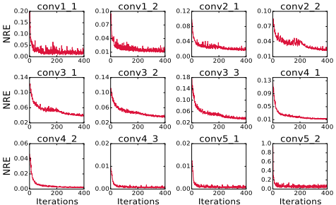
We provide empirical evidences on the convergence of the proposed method in Figure 6. Because NRE is the optimization objective when pruning single layer, we plot the NRE curves with respect to iterations in all layers except for the last one of VGGNet. It can be observed from Figure 6 that all the NRE curves become flatten after 400 iterations. In conv5 1 and conv5 2, the NRE curves do not drop even after dozens of iterations. These evidences show that our algorithm can converge very fast.
Next we explore whether the selected channels are really important after convergence. To this end, we visualize all 96 filters in the first convolutional layer (conv1) of AlexNet, which is pruned by the proposed method as shown in Figure 5. Note that a filter is a collection of all incoming weights of a channel and the proposed method can prune 24 channels in conv1. The filters connected to 24 pruned channels are shown with black boxes. We can see that filters with black boxes contain very little information, which indicates that the proposed method prunes the least important channels.
Validity of NRE
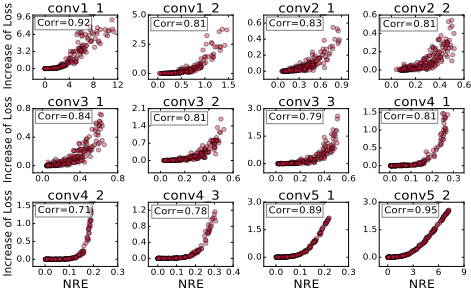
We also explore the correlation between the layer-wise NRE and the entire loss (i.e., the loss from output layer), which is important to the validity of layer-wise pruning and is rarely explored in previous works. For this purpose, we randomly delete channels in one layer of the baseline VGGNet model, and record the NRE of the next layer as well as the increase of the entire loss. Then, we plot the increase curves of the entire loss with respect to the NRE in all layers except for the last one of VGGNet in Figure 7. Unsurprisingly, these two variables show a strong positive correlation, and the correlation coefficient is even larger than 0.9 in some layers (e.g., conv1 1 and conv5 2). These facts demonstrate that minimizing the layer-wise NRE is reasonable.
4 Conclusion
In this paper, we propose a new layer-wise neuron pruning method to accelerate the deep models and reduce their memory usage. By extracting a 3-layer subnetwork, the proposed method formulates one single layer neuron pruning as a constrained optimization problem, i.e., minimizing the layerwise nonlinear reconstruction error with a limited number of neurons, and then solves it by adopting an iterative greedy selection algorithm. Experiments on benchmark DNN models show that the proposed method can reach state-of-the-art compression rate and speedup with an acceptable loss of accuracy. In the future, we will generalize the proposed method to multi-branch convolutional neural networks like ResNet or other types of neural networks like RNN.
@inproceedings{ijcai2018p318,
  title     = {Efficient DNN Neuron Pruning by Minimizing Layer-wise Nonlinear Reconstruction Error},
  author    = {Jiang, Chunhui and Li, Guiying and Qian, Chao and Tang, Ke},
  booktitle = {Proceedings of the Twenty-Seventh International Joint Conference on
               Artificial Intelligence, {IJCAI-18}},
  publisher = {International Joint Conferences on Artificial Intelligence Organization},
  editor    = {Jérôme Lang},
  pages     = {2298--2304},
  year      = {2018},
  month     = {7},
  note      = {Main track},
  doi       = {10.24963/ijcai.2018/318},
  url       = {https://doi.org/10.24963/ijcai.2018/318},
}
TY - CPAPER TI - Efficient DNN Neuron Pruning by Minimizing Layer-wise Nonlinear Reconstruction Error AU - Jiang, Chunhui AU - Li, Guiying AU - Qian, Chao AU - Tang, Ke T2 - Proceedings of the Twenty-Seventh International Joint Conference on Artificial Intelligence, IJCAI-18 PB - International Joint Conferences on Artificial Intelligence Organization PY - 2018 SP - 2298 EP - 2304 DO - 10.24963/ijcai.2018/318 UR - https://doi.org/10.24963/ijcai.2018/318 ER -Copied
Machine-readable versions of this paper, for tools and AI agents:





