
A Normalized Convolutional Neural Network for Guided Sparse Depth Upsampling
Proceedings of the Twenty-Seventh International Joint Conference on Artificial Intelligence. Main track. Pages 2283-2290.
https://doi.org/10.24963/ijcai.2018/316
Keywords
- Machine Learning: Deep Learning
- Computer Vision: Computer Vision
- Computer Vision: 2D and 3D Computer Vision
Abstract
Guided sparse depth upsampling aims to upsample an irregularly sampled sparse depth map when an aligned high-resolution color image is given as guidance. When deep convolutional neural networks (CNNs) become the optimal choice to many applications nowadays, how to deal with irregular and sparse data still remains a non-trivial problem. Inspired by the classical normalized convolution operation, this work proposes a normalized convolutional layer (NCL) implemented in CNNs. Sparse data are therefore explicitly considered in CNNs by the separation of both data and filters into a signal part and a certainty part. Based upon NCLs, we design a normalized convolutional neural network (NCNN) to perform guided sparse depth upsampling. Experiments on both indoor and outdoor datasets show that the proposed NCNN models achieve state-of-the-art upsampling performance. Moreover, the models using NCLs gain a great generalization ability to different sparsity levels.
- [Abadi et al., 2016] M. Abadi, A. Agarwal, P. Barham, E. Brevdo, Z. Chen, C. Citro, G. Corrado, A. Davis, J. Dean, M. Devin, et al. Tensorflow: Large-scale machine learning on heterogeneous distributed systems. arXiv preprint arXiv:1603.04467, 2016.
- [Chen et al., 2017] X. Chen, H. Ma, J. Wan, B. Li, and T. Xia. Multi-view 3d object detection network for au- tonomous driving. In CVPR, 2017.
- [Dahl et al., 2017] R. Dahl, M. Norouzi, and J. Shlens. Pixel recursive super resolution. In ICCV, 2017.
- [Diebel and Thrun, 2006] J. Diebel and S. Thrun. An appli- cation of markov random fields to range sensing. In NIPS, 2006.
- [Dong et al., 2016] C. Dong, C. Loy, and X. He, K.and Tang. Image super-resolution using deep convolutional net- works. IEEE transactions on pattern analysis and machine intelligence, 38(2):295-307, 2016.
- [Ferstl et al., 2013] D. Ferstl, C. Reinbacher, R. Ranftl, M. Rüther, and H. Bischof. Image guided depth upsam- pling using anisotropic total generalized variation. In ICCV, 2013.
- [Gaidon et al., 2016] A.. Gaidon, Q Wang, Y. Cabon, and E. Vig. Virtual worlds as proxy for multi-object tracking analysis. In CVPR, 2016.
- [Geiger et al., 2012] A. Geiger, P. Lenz, and R. Urtasun. Are we ready for autonomous driving? the kitti vision bench- mark suite. In CVPR, 2012.
- [Glorot and Bengio, 2010] X. Glorot and Y. Bengio. Under- standing the difficulty of training deep feedforward neural networks. In AISTATS, 2010.
- [Godard et al., 2017] C. Godard, O. Mac Aodha, and G. Brostow. Unsupervised monocular depth estimation with left-right consistency. In CVPR, 2017.
- [Ham et al., 2015] B. Ham, M. Cho, and J. Ponce. Robust image filtering using joint static and dynamic guidance. In CVPR, 2015.
- [Harrison and Newman, 2010] Alastair Harrison and Paul Newman. Image and sparse laser fusion for dense scene reconstruction. In Field and Service Robotics, pages 219- 228. Springer, 2010.
- [Hou and Andrews, 1978] H. Hou and H. Andrews. Cubic splines for image interpolation and digital filtering. IEEE Transactions on acoustics, speech, and signal processing, 26(6):508-517, 1978.
- [Hui et al., 2016] T. Hui, C. Loy, and X. Tang. Depth map super-resolution by deep multi-scale guidance. In ECCV, 2016.
- [Kim et al., 2016] J. Kim, J. Lee, and Lee K. Accurate image super-resolution using very deep convolutional networks. In CVPR, 2016.
- [Kingma and Ba, 2014] D. Kingma and J. Ba. Adam: A method for stochastic optimization. In ICLR, 2014. [Knutsson and Westin, 1993]
- H. Knutsson and C.-F. Westin. Normalized and differential convolution methods for inter- polation and filtering of incomplete and uncertain data. In CVPR, 1993.
- [Kuznietsov et al., 2017] Y. Kuznietsov, J. Stückler, and B. Leibe. Semi-supervised deep learning for monocular depth map prediction. In CVPR, 2017.
- [Laina et al., 2016] I.
- Laina, C. Rupprecht, V. Belagiannis, F. Tombari, and N. Navab. Deeper depth prediction with fully convolutional residual networks. In International Conference on 3D Vision, 2016.
- [Li et al., 2016a] B. Li, T. Zhang, and T. Xia. Vehicle de- tection from 3d lidar using fully convolutional network. Robotics: Science and Systems, 2016.
- [Li et al., 2016b] Y. Li, J. Huang, N. Ahuja, and M. Yang. Deep joint image filtering. In ECCV, 2016.
- [Ma and Karaman, 2018] F. Ma and S. Karaman. Sparse-to- dense: Depth prediction from sparse depth samples and a single image. In ICRA, 2018.
- [McCormac et al., 2017] J. McCormac, A. Handa, S. Leutenegger, and A. Davison. Scenenet rgb-d: 5m photorealistic images of synthetic indoor trajectories with ground truth. In ICCV, 2017.
- [Min et al., 2012] D. Min, J. Lu, and M. Do. Depth video en- hancement based on weighted mode filtering. IEEE Trans- actions on Image Processing, 21(3):1176-1190, 2012.
- [Park et al., 2011] J. Park, H. Kim, Y. Tai, M. Brown, and I. Kweon. High quality depth map upsampling for 3d-tof cameras. In ICCV, 2011.
- [Petschnigg et al., 2004] G. Petschnigg, R. Szeliski, M. Agrawala, M. Cohen, H. Hoppe, and K. Toyama. Digital photography with flash and no-flash image pairs. ACM transactions on graphics, 23(3):664-672, 2004.
- [Riegler et al., 2016a] G. Riegler, D. Ferstl, M. Rüther, and H. Bischof. A deep primal-dual network for guided depth super-resolution. In BMVC, 2016.
- [Riegler et al., 2016b] G. Riegler, M. Rüther, and H. Bischof. Atgv-net: accurate depth super-resolution. In ECCV, 2016.
- [Tomasi and Manduchi, 1998] C. Tomasi and R. Manduchi. Bilateral filtering for gray and color images. In ICCV, 1998.
- [Uhrig et al., 2017] J. Uhrig, N. Schneider, L. Schneider, U. Franke, T. Brox, and A. Geiger. Sparsity invariant cnns. In International Conference on 3D Vision, 2017.
- [Velodyne, 2018] Velodyne. http://velodynelidar.com/hdl- 64e.html, 2018. Link
- [Yang et al., 2010] J. Yang, J. Wright, T. Huang, and Y. Ma. Image super-resolution via sparse representation. IEEE transactions on image processing, 19(11):2861-2873, 2010.
- [Zweig and Wolf, 2017] S. Zweig and L. Wolf. Interponet, a brain inspired neural network for optical flow dense inter- polation. In CVPR, 2017.
References were extracted automatically from the PDF and may contain errors.
Full text extracted automatically from the PDF; figures, tables and equations may differ. The PDF is the version of record.
1 Introduction
Guided sparse depth upsampling aims to reconstruct a dense depth map from irregularly sampled sparse measurements under the guidance of a high-resolution color image. This task has received considerable attention since the joint use of 3D laser scanners and visual cameras became popular in autonomous driving. Due to the limitation of hardware development, state-of-the-art range sensors still acquire much lower-resolution data when compared to visual images. Even for Velodyne HDL-64e [Velodyne, 2018], when projecting sparse 3D point clouds into an aligned 2D image, it obtains only approximately 5% valid depth values in the projected image. Such a high sparsity level makes it challenging to perform subsequent tasks such as RGB-D based object detection and road scene understanding.
Guided depth upsampling has been studied for decades. Traditional methods often rely on either local or global techniques. The former, such as joint bilateral filtering methods [Tomasi and Manduchi, 1998; Petschnigg et al., 2004], predicts unknown depth values according to their neighbourhood. The latter, e.g. Markov random fields [Diebel and Thrun, 2006; Park et al., 2011], formulates the task as a global energy minimization problem. In these methods, structral similarity is measured in terms of hand-crafted features, which limit the upsampling performance. Recently, deep convolutional neural networks (CNNs) [Riegler et al., 2016a; Hui et al., 2016; Li et al., 2016b] are applied to this task. But they all assume that input data is complete and defined on regular 2D grids. When applying CNNs for guided sparse depth upsampling, we have to tackle a particular problem. That is, how to deal with irregular and sparse inputs in CNNs?
∗The corresponding author
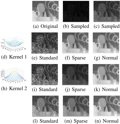
For this problem, a naive solution is to fill missing values with 0 and feed the input into standard CNNs. When the input data are dependent and the underlying distribution keeps the same, the standard CNNs are able to deduce the missing values. However, these models lack the generalization ability when the sparsity level is changed. To overcome this disadvantage, Uhrig et al. [Uhrig et al., 2017] propose a sparse convolutional layer in CNNs that takes the certainty of data into account, by which sparsity invariance is achieved. Our work is close to theirs but inspired by normalized convolution [Knutsson and Westin, 1993], which was proposed for filtering incomplete or uncertain data in 1990s. Figure 1 illustrates some typical results obtained by applying three convolution operations, i.e. standard, sparse, and normalized convolutions, directly on sparse depth maps when using different kernels and different sampling rates. The results show that normalized convolution outperforms the others no matter which kernel or sampling rate is taken.
The above phenomenon draws our attention to the factors that might affect the performance of sparse depth upsampling. We think there are three key factors: (1) Filter. Better filters, better performance. That's why learning filters in CNNs can be expected to outperform most explicitly defined filtering methods. (2) Convolution operation. The conducted experiments show that normalized convolution alone, even if it is not used in the CNN framework, can get acceptable upsampling results. (3) Extra information for guidance. The integration of a high-resolution color image may help to recover high frequency components in depth maps based on the co-occurrence assumption.
Therefore, in this work we opt to combine the advantages of CNNs and normalized convolution to perform the sparse depth upsampling task, while integrating high-resolution color images as guidance. To better perform the guided sparse depth upsampling task, we make the following contributions:
- Based upon normalized convolution, we propose a normalized convolutional layer (NCL) implemented in CNNs to deal with sparse and irregular input data. Different from the existing sparse convolution, NCL takes both the certainty of data and the applicability of filters into account. As evidenced by experiments, our trained model not only gains the ability to adapt to various sparsity levels, but also achieves increasing performance when more certain data are input.
- Base upon NCL, we propose a new architecture named normalized convolutional neural network (NCNN) to perform guided sparse depth upsampling. The frontend of NCNN consists of two streams: one uses standard convolutional layers to cope with a dense guidance image, and the other applies NCLs to deal with a sparse depth map. The backend of CNN fuses the outputs of two streams together to predict the dense upsampling result. Experiments on various datasets demonstrate that our approach outperforms the state-of-the-arts.
2 RelatedWork
Our work is most related to the techniques dealing with sparse inputs and depth upsampling. Thus, this section makes a brief review on these aspects.
2.1 CNNs with Sparse Inputs
The input of standard CNN models is supposed to be dense. How to deal with sparse and irregular data in CNNs is a nontrivial problem. A naive solution is set missing values to be 0 and feeds the input into a standard CNN, as done in [Chen et al., 2017] [Li et al., 2016a]. Another alternative way is passing the sparse input together with an additional binary certainty mask to CNNs [Zweig and Wolf, 2017]. Both options leave the standard convolutional networks unchanged. An exception is the work done by Uhrig et al. [Uhrig et al., 2017], who propose a sparse convolutional layer to consider data's certainty within the convolution operation.
Our work is close to [Uhrig et al., 2017] but inspired by normalized convolution (NC) [Knutsson and Westin, 1993]. NC is a classical technique proposed to filter sparse or incomplete data by separating both data and convolutional operator into a signal part and a certainty part. We implement NC as a layer in CNNs for sparse inputs. Benefited from the least square optimality property that NC holds, our model gains better performance.
2.2 Depth Upsampling and Prediction
According to whether we use extra information for guidance or not, depth upsampling can be classified into non-guided and guided techniques.
Non-guided depth upsampling is close to image superresolution. Early methods are often based on interpolation [Hou and Andrews, 1978], sparse representation [Yang et al., 2010] and other traditional techniques. Recently, deep learning based methods have demonstrated a great success in depth [Riegler et al., 2016b; Uhrig et al., 2017] or color [Dong et al., 2016; Kim et al., 2016; Dahl et al., 2017] image super-resolution. Except [Uhrig et al., 2017], all above mentioned techniques cope with regular low-resolution images and have no concerns particular to irregularly sampled sparse data.
Guided depth upsampling takes a high-resolution image as guidance. It is based on an observation that depth discontinuities often co-occur with color or intensity changes. Traditional methods mainly rely on local filtering techniques such as joint bilateral filtering [Tomasi and Manduchi, 1998; Petschnigg et al., 2004], and global optimization techiniques such as Markov random fields [Diebel and Thrun, 2006; Park et al., 2011]. These methods are able to deal with both regularly and irregularly sampled data, but they use hand-crafted features that limit their performance. In recent years, researchers have come up with various deep learning methods [Riegler et al., 2016a; Hui et al., 2016; Li et al., 2016b] for guided upsampling. Again, these methods only deal with regular low-resolution depth maps.
Depth prediction from a monocular color image based on deep learning methods [Laina et al., 2016; Godard et al., 2017] is attracting considerable attention nowadays. In addition, sparse laser measurements are also integrated by Kuznietsov et al. [Kuznietsov et al., 2017] and Ma et al. [Ma and Karaman, 2018] to regularize depth prediction results. All above depth prediction methods can be viewed as a domain transfer problem that regresses depth values from color/intensity values. They rely more on color images but take sparse depth maps as guidance. Conversely, color images are used to guide depth upsampling in our work.
3 The ProposedMethod
In this section, we first introduce the concept of normalized convolution for the purpose of self-containedness. We then present the implementation of normalized convolution as a layer in CNNs, upon which a normalized convolutional neural network (NCNN) is designed for guided depth upsampling.
3.1 Normalized Convolution
Normalized convolution was first introduced by Knutsson and Westin [Knutsson and Westin, 1993]. It is based on the separation of both data and operator into a signal part and a certainty part, through which irregular sampled data can be handled by setting the certainty to 1 in the sampling points and 0 elsewhere. Therefore, it is applicable to perform operations on incomplete or uncertain data.
Let u be the global spatial coordinate and i be the coordinate in a local window. X(u) denotes a tensor representing an input signal. c(u) is a positive scalar value indicating the certainty of X(u). When considering a convolution, we use a tensor B(i) to represent the filter basis and a positive scalar value a(i) to represent the applicability of B(i).
Definition of Standard Convolution
Following the definitions in [Knutsson and Westin, 1993], a generalized form of convolution is defined by
where ⊙ denotes some multilinear operation (in standard convolution this operation is scalar multiplication). For compactness, it can be written as
whereˆover the multilinear operation indicates that the operation is involved in the convolution.
Definition of Normalized Convolution
Normalized convolution of aB and cX is then defined by
where
in which · denotes standard scalar multiplication and ∗ denotes complex conjugate.
Property of Normalized Convolution
As shown in [Knutsson and Westin, 1993], normalized convolution produces a description of the neighbourhood that is optimal in a least square sense. Again, for self-containedness, we show this property here.
Let us consider a neighbourhood d. If a set of basis functions, denoted by a matrix B, are given, we normally get
which approximately represents the neighbourhood. By minimizing the least square error ||d′ - d||22 , we get the coefficients x to be:
Considering a weighted least square error ||W(d′ - d)||22 , in which W is a diagonal weighing matrix, the error is minimized by choosing x to be:
It can be rewritten and split into two parts as follows:
in which N and D are shown to be identical to the corresponding terms defined in normalized convolution.
In normalized convolution, the diagonal weighing matrix for a neighbourhood centered on u0 is given by
which depends on the certainty of data and the applicability of the convolution kernel. Therefore, normalized convolution can be viewed as a method for obtaining a local weighted least square error description of the input signal. When better applicability or more certain data are considered, we can reconstruct the original dense signal better.
3.2 Normalized Convolutional Layer
Standard convolutional layer is a key component for CNNs to achieve giant success. It inspires us to implement normalized convolution as a layer in CNNs to deal with irregularly sampled images. To this end, we consider a 2D sparse depth map as the input signal, then the global and local spatial coordinates can be explicitly represented as u = (u, v) and i = (i, j), respectively. We further use the set of impulses located at each pixel as the basis to represent the convolution filter. Then, normalized convolution can be rewritten as:
Here, regarding to the filter basis that we chose, we get w(i, j) = a(i, j)B(i, j) = a(i, j). The filter size is (2K + 1)×(2K+1). b is a bias commonly added in a convolutional layer and ϵ is a small value placed to avoid dividing by zero.
For dealing with 2D sparse depth maps, another technique named sparse convolution [Uhrig et al., 2017] was proposed recently. It considers the certainty of the input signal but has no concern on the applicability of the filters. It is defined in the form of
In contrast to normalized convolution, the above defined sparse convolution does not hold the least square optimality property. Moreover, normalized convolution can preserve the range of the signal during convolution while sparse convolution can not.
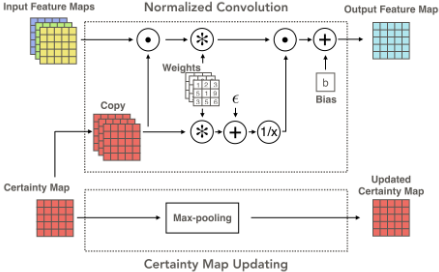
When implementing normalized convolution as a layer in CNNs, we take a 2D signal and its corresponding certainty map as the inputs. The 2D input signal might be a singlechannel sparse depth map or multi-channel sparse feature maps. The corresponding certainty map is initially set to be 1 at the measured pixels and 0 otherwise. As a layer used in CNNs, it is necessary to update the certainty map when the measured information are propagated to neighbours during convolution, and pass the updated certainty map into next layers. The update can be implemented via the max-pooling operation defined by
which sets the certainty of the pixels to 1 if at least one measured pixel is into the filter and 0 otherwise.
Figure 3 illustrates the network structure of our normalized convolutional layer. As mentioned above, it takes a 2D signal and the associated certainty map as the inputs, and outputs a feature map and an updated certainty map. Moreover, it consists of two streams: one implements the normalized convolution defined in Equation (11) and the other is for certainty map update.
3.3 NCNN for Guided Depth Upsampling
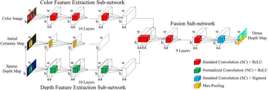
Based upon above implementations, we propose a normalized convolutional neural network (NCNN) to perform guided sparse depth upsampling. Figure 2 illustrates the entire architecture. It consists of three major components: color feature extraction sub-network, depth feature extraction subnetwork, and feature fusion sub-network.
The Color Feature Extraction Sub-network
This sub-network takes a guidance image, which is dense and in color, as the input. When designing its architecture, we have the following concerns: (1) As validated in many applications, standard convolutional layers (SCLs) are powerful to extract features from regular images. Thus, this sub-network uses a stack of SCLs for feature extraction. (2) In contrast to other applications such as image classification or object detection, the depth upsampling task needs finer scale features. Thus, instead of using large size filers and max-pooling operations, each convolutional layer adopts filters in the size of 3 × 3 and is followed only by ReLU activations but no max-poolings. Moreover, zero padding is used before convolutions to keep the size of all feature maps the same as the input. (3) As shown in [Kim et al., 2016], taking large context into account benefits super-resolution results. Therefore this sub-network empirically stacks 10 convolutional layers to gain large receptive fields.
The Depth Feature Extraction Sub-network
This sub-network takes a sparse depth map and its certainty map as the inputs. This sub-network has the same architecture as the previous one, but replacing all SCLs by our normalized convolutional layers. The NCLs play two roles: on one hand, they are able to extract features directly from an irregularly sampled sparse depth map; on the other hand, the NCLs also perform interpolation or upsampling for sparse data so that the produced feature maps are dense.
The Feature Fusion Sub-network
This sub-network takes the concatenation of the outputs from previous two streams as the input. Considering that the feature maps from both streams are dense, we therefore use SCLs the same as in the color stream to perform feature fusion. When choosing the layer number, we find out that a shallow architecture is prone to transfer unnecessary structure details from the guidance image to depth prediction results. A deep architecture can highly reduce such effects but increases computational costs. Thus, we experimentally set 9 layers for fusion. In the end a 1 × 1 convolutional layer followed by Sigmoid is connected to predict a dense depth map.
Network Training
In the training phase, we are given N training samples {Disparse , I i color , Digt }Ni=1 , in which Disparse denotes a sparse depth map, I i color represents the aligned color image for guidance, and Digt is the ground truth dense depth map. Let F represent the mapping function over the whole network and ω be the collection of all network parameters, then the output of the network Dipred , which is the predicted dense depth map, is represented by
Then, we define the entire training loss function as below.
where λ is a scalar to balance two terms. The former term is a square error of all pixels and the L2 regularization term of ω is added to avoid overfitting. The whole network is trained endto-end. The loss function is optimized by ADAM [Kingma and Ba, 2014].
4 Experimental Results
In this section, we first introduce implementation details, together with the datasets and the metric used for evaluation. Experimental results evaluated on different datasets are then demonstrated to validate the effectiveness of our approach.
4.1 Experimental Setup
Our approach is implemented based on Tensorflow [Abadi et al., 2016]. In experiments, we do not use any pre-trained models but initialize weight parameters via Xavier [Glorot and Bengio, 2010] and set the initial bias to be 0. We empirically set the hyper-parameter λ in Equation (15) as 10-4 by referring to other models [Kim et al., 2016] and fix it throughout all the experiments. We train all experiments enough epochs till convergence with a batch size of 4. Learning rate is initially set to 10-4 .
In order to have dense depth maps, we conduct our experiments on two synthetic datasets: SceneNet RGB-D [McCormac et al., 2017] and Virtual KITTI [Gaidon et al., 2016].
- SceneNet RGB-D is a dataset for indoor scenes. It contains 5 million rendered RGB-D images in the resolution of 320 × 240. In experiments, we randomly sample
15000 training images from its training set and 2000 test images from its validation set.
- Virtual KITTI is an outdoor dataset synthetically cloned from the real-world KITTI benchmark [Geiger et al., 2012]. It contains 21260 RGB-D images with 5 sequences and 10 different rendering variations. In our experiments, we use 8 variations by leaving out fog and rain weather scenarios. 4 sequences are chosen for training and 1 sequence for testing, by which we get 13432 training samples and 3576 test images.
Both datasets provide us with dense depth maps and aligned color images. For experiments we synthetically generate sparse depth maps by randomly sampling a percentage of points from the provided depth maps. Experimental results are evaluated with respect to root-mean-square error (RMSE).
4.2 Ablation Experiments
We run a number of ablation experiments to analyze our proposed models. To investigate the effectiveness of NCL, we compare our models with those replacing NCLs with either standard convolutional layers or sparse convolutional layers. These models are, respectively, denoted using the suffixes ' Norm', ' Stand' and ' Sparse'. To investigate the effectiveness of guidance, we compare our full model with the one without the color feature extraction stream, and use 'G' and 'NG' to distinguish them. To check the effectiveness of NCNN architecture, we compare our 'NG' models with SparseConvNet [Uhrig et al., 2017], which is a network architecture designed for non-guided sparse depth upsampling.
In experiments, we train all models at a single sampling rate (5%) and test them at various rates. Experiments are conducted on both datasets, from which consistent phenomena can be observed. We present the results on the SceneNet RGB-D dataset in Table 1 and the results on the Virtual KITTI dataset in Table 2. Experimental results on both datasets consistently demonstrate the following phenomena: (1) Contrary to the results in [Uhrig et al., 2017], in our experiments, the models using standard convolution gain the best performance when test data has the same or close sampling rate. But their performance degenerates dramatically as the sampling rate goes up, indicating that these models lack of generalization ability. (2) Both normalized convolution and sparse convolution have great generalization abilities. The least square optimality of NC can be viewed as placing an implicit constraint on each NCL, which makes the NCL-based models achieve better upsampling performance. Moreover, although the distribution of test data is quite different from that of training data, NC achieves increasing performance as more certain data are input. (3) The models using guidance information perform better than those without guidance. (4) The comparison between our 'NG' models and the SparseConvNet models show that our network architecture is superior.
In addition, we also tried to compare the training efficiency of three convolutional operations by checking the curves of training loss. In our experiments all the models converge fast and the one using NCL only shows a slight advantage.
| ❤❤❤❤❤❤❤❤❤❤ Models Sampling rate | 5% | 10% | 20% | 30% | 40% | 50% | 60% | 70% | 80% | 90% | 100% |
|---|---|---|---|---|---|---|---|---|---|---|---|
| SparseConvNet Stand | 2.115 | 1.722 | 2.053 | 3.029 | 4.483 | 6.195 | 7.973 | 9.798 | 11.837 | 14.333 | 17.895 |
| SparseConvNet Sparse | 2.145 | 1.777 | 1.704 | 1.690 | 1.687 | 1.685 | 1.684 | 1.683 | 1.683 | 1.683 | 1.683 |
| SparseConvNet Norm | 1.947 | 1.576 | 1.420 | 1.372 | 1.350 | 1.337 | 1.329 | 1.323 | 1.319 | 1.316 | 1.313 |
| NCNN NG Stand | 1.774 | 1.323 | 1.165 | 1.238 | 1.476 | 1.922 | 2.686 | 3.873 | 5.554 | 7.861 | 11.618 |
| NCNN NG Sparse | 1.944 | 1.510 | 1.342 | 1.296 | 1.281 | 1.272 | 1.266 | 1.264 | 1.262 | 1.260 | 1.259 |
| NCNN NG Norm | 1.833 | 1.362 | 1.155 | 1.092 | 1.070 | 1.057 | 1.048 | 1.043 | 1.039 | 1.036 | 1.034 |
| NCNN G Stand | 1.166 | 1.017 | 0.945 | 1.009 | 1.200 | 1.508 | 1.879 | 2.252 | 2.571 | 2.808 | 2.939 |
| NCNN G Sparse | 1.265 | 1.120 | 1.057 | 1.045 | 1.043 | 1.044 | 1.045 | 1.045 | 1.046 | 1.047 | 1.047 |
| NCNN G Norm | 1.212 | 1.069 | 0.985 | 0.955 | 0.939 | 0.930 | 0.924 | 0.919 | 0.916 | 0.914 | 0.912 |
| ❤❤❤❤❤❤❤❤❤❤ Models Sampling rate | 5% | 10% | 20% | 30% | 40% | 50% | 60% | 70% | 80% | 90% | 100% |
|---|---|---|---|---|---|---|---|---|---|---|---|
| SparseConvNet Stand | 2.344 | 2.033 | 1.944 | 2.051 | 2.241 | 2.357 | 2.449 | 3.155 | 5.672 | 11.021 | 16.632 |
| SparseConvNet Sparse | 2.482 | 2.285 | 2.202 | 2.174 | 2.160 | 2.151 | 2.145 | 2.140 | 2.136 | 2.132 | 2.130 |
| SparseConvNet Norm | 2.350 | 2.012 | 1.799 | 1.725 | 1.690 | 1.669 | 1.656 | 1.647 | 1.640 | 1.634 | 1.630 |
| NCNN NG Stand | 2.129 | 1.796 | 1.606 | 1.576 | 1.611 | 1.695 | 1.830 | 1.995 | 2.148 | 2.254 | 2.289 |
| NCNN NG Sparse | 2.290 | 2.000 | 1.851 | 1.808 | 1.790 | 1.781 | 1.775 | 1.771 | 1.768 | 1.766 | 1.764 |
| NCNN NG Norm | 2.172 | 1.839 | 1.638 | 1.569 | 1.534 | 1.513 | 1.500 | 1.492 | 1.486 | 1.482 | 1.480 |
| NCNN G Stand | 1.153 | 0.993 | 0.895 | 0.887 | 0.989 | 1.235 | 1.586 | 1.972 | 2.348 | 2.674 | 2.821 |
| NCNN G Sparse | 1.298 | 1.195 | 1.173 | 1.173 | 1.175 | 1.177 | 1.179 | 1.180 | 1.181 | 1.182 | 1.182 |
| NCNN G Norm | 1.186 | 1.041 | 0.982 | 0.970 | 0.965 | 0.963 | 0.962 | 0.961 | 0.960 | 0.959 | 0.959 |
4.3 Visualization of Feature Maps
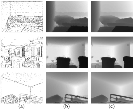
In our network, we use standard convolutional layers to extract features from dense RGB images while employ the proposed NCLs to extract features and perform upsampling for sparse dense maps, and use standard convolution again in the fusion sub-network. It is interesting to see whether such design is appropriate. To this end, we demonstrate some typical intermediate features generated in different sub-networks in Figure 6. From it we can observe that the feature maps obtained from the color feature extraction sub-network provide structured information, while those maps from the depth sub-network seem more like coarsely upsampled dense depth maps. The fusion of both transfers the structured features from color images to recover high frequency components of depth maps. These phenomena provide supporting evidence for our network design.
4.4 Comparison to Other Methods
We then compare our full model 'NCNN G Norm' to other guided depth upsampling techniques, including 5 representative non-deep-learning methods: JBF [Petschnigg et al., 2004], MRF [Harrison and Newman, 2010], WMF [Min et al., 2012], TGV [Ferstl et al., 2013], SDF [Ham et al., 2015], and 1 deep learning approach DJF [Li et al., 2016b]. Table 3 and 4 report the experimental results at five sampling rates (5%, 20%, 50%, 80% and 100%) on both datasets. For training based methods, experiments are trained and tested at the same rate. For comparison, we also include the results of 'NCNN G Norm' trained at 5%while tested at all the rates.
| ❤❤❤❤❤❤❤❤❤❤ Methods Sampling rate | 5% | 20% | 50% | 80% | 100% |
|---|---|---|---|---|---|
| JBF[Petschnigg et al., 2004] | 1.509 | 1.156 | 1.036 | 0.993 | 0.975 |
| MRF[Harrison and Newman, 2010] | 1.723 | 1.187 | 0.853 | 0.648 | 0.529 |
| WMF[Min et al., 2012] | 1.680 | 1.261 | 1.089 | 1.020 | 0.989 |
| TGV[Ferstl et al., 2013] | 1.671 | 1.030 | 0.665 | 0.382 | 0.000 |
| SDF[Ham et al., 2015] | 2.006 | 1.296 | 0.868 | 0.570 | 0.390 |
| DJF[Li et al., 2016b] | 1.842 | 1.251 | 0.922 | 0.640 | 0.176 |
| NCNN G Norm⋄ (ours) | 1.212 | 0.985 | 0.930 | 0.916 | 0.912 |
| NCNN G Norm(ours) | 1.212 | 0.930 | 0.714 | 0.465 | 0.103 |
| ❤❤❤❤❤❤❤❤❤❤ Methods Sampling rate | 5% | 20% | 50% | 80% | 100% |
|---|---|---|---|---|---|
| JBF[Petschnigg et al., 2004] | 2.152 | 1.439 | 1.197 | 1.123 | 1.096 |
| MRF[Harrison and Newman, 2010] | 2.380 | 1.602 | 1.089 | 0.768 | 0.563 |
| WMF[Min et al., 2012] | 2.356 | 1.606 | 1.329 | 1.241 | 1.208 |
| TGV[Ferstl et al., 2013] | 2.236 | 1.493 | 0.991 | 0.556 | 0.000 |
| SDF[Ham et al., 2015] | 2.888 | 1.782 | 1.147 | 0.774 | 0.718 |
| DJF[Li et al., 2016b] | 2.113 | 1.425 | 0.874 | 0.631 | 0.189 |
| NCNN G Norm⋄ (ours) | 1.186 | 0.982 | 0.963 | 0.960 | 0.959 |
| NCNN G Norm(ours) | 1.186 | 0.832 | 0.527 | 0.347 | 0.072 |
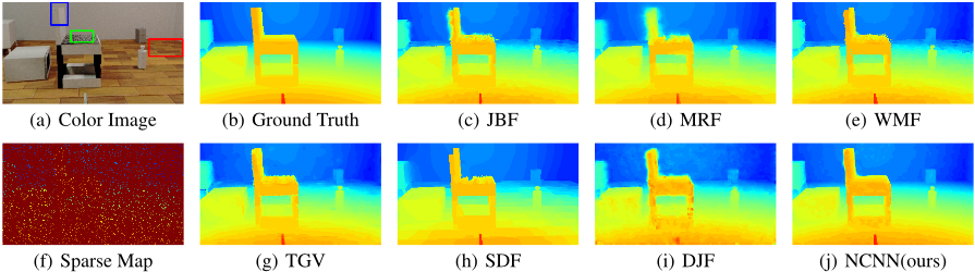

From Table 3 and 4 we get the following observations: (1) When training and testing at the same sampling rate, our proposed model outperforms both traditional and deep learning methods in most cases, especially when the sampling rate is low. (2) Even if our model is trained only at 5% sampling rate, its performance at other sampling rates is still competitive to the others. Figure 4 illustrates qualitative results obtained by these methods on the SceneNet RGB-D dataset. As shown in the regions marked by green and red boxes, our approach can better prevent from transferring unnecessary structural details from guidance to the upsampled depth map. On the other hand, our approach keeps object boundaries sharper, as shown in the region within the blue box. The qualitative results obtained by these methods on the Virtual KITTI dataset are also presented in Figure 5. The region marked by the blue box shows that our approach can keep object boundaries sharper and recover slim objects (the pole) better. Our approach also prevent unnecessary structural details, see the regions marked by the red box.
5 Conclusion
Inspired by the classical normalized convolution operation, in this work we proposed a normalized convolutional layer in CNNs to deal with irregular and sparse data, and presented a normalized convolutional neural network to perform guided sparse depth upsampling. Experiments on both indoor and outdoor datasets show that our NCNN models outperform other guided depth upsampling methods. Moreover, supported by the least square optimality property of NC, the models using NCLs gain a great generalization ability to different levels of sparsity. This ability is desirable in applications where range sensor configurations might be changed.
Acknowledgments
This work was supported in part by the Natural Science Foundation of Zhejiang Province, China under Grant LY17F010007.
@inproceedings{ijcai2018p316,
  title     = {A Normalized Convolutional Neural Network for Guided Sparse Depth Upsampling},
  author    = {Hua, Jiashen and Gong, Xiaojin},
  booktitle = {Proceedings of the Twenty-Seventh International Joint Conference on
               Artificial Intelligence, {IJCAI-18}},
  publisher = {International Joint Conferences on Artificial Intelligence Organization},
  editor    = {Jérôme Lang},
  pages     = {2283--2290},
  year      = {2018},
  month     = {7},
  note      = {Main track},
  doi       = {10.24963/ijcai.2018/316},
  url       = {https://doi.org/10.24963/ijcai.2018/316},
}
TY - CPAPER TI - A Normalized Convolutional Neural Network for Guided Sparse Depth Upsampling AU - Hua, Jiashen AU - Gong, Xiaojin T2 - Proceedings of the Twenty-Seventh International Joint Conference on Artificial Intelligence, IJCAI-18 PB - International Joint Conferences on Artificial Intelligence Organization PY - 2018 SP - 2283 EP - 2290 DO - 10.24963/ijcai.2018/316 UR - https://doi.org/10.24963/ijcai.2018/316 ER -Copied
Machine-readable versions of this paper, for tools and AI agents:





