
Generative Adversarial Positive-Unlabelled Learning
Proceedings of the Twenty-Seventh International Joint Conference on Artificial Intelligence. Main track. Pages 2255-2261.
https://doi.org/10.24963/ijcai.2018/312
Keywords
- Machine Learning: Semi-Supervised Learning
- Machine Learning: Learning Generative Models
Abstract
In this work, we consider the task of classifying binary positive-unlabeled (PU) data. The existing discriminative learning based PU models attempt to seek an optimal reweighting strategy for U data, so that a decent decision boundary can be found. However, given limited P data, the conventional PU models tend to suffer from overfitting when adapted to very flexible deep neural networks. In contrast, we are the first to innovate a totally new paradigm to attack the binary PU task, from perspective of generative learning by leveraging the powerful generative adversarial networks (GAN). Our generative positive-unlabeled (GenPU) framework incorporates an array of discriminators and generators that are endowed with different roles in simultaneously producing positive and negative realistic samples. We provide theoretical analysis to justify that, at equilibrium, GenPU is capable of recovering both positive and negative data distributions. Moreover, we show GenPU is generalizable and closely related to the semi-supervised classification. Given rather limited P data, experiments on both synthetic and real-world dataset demonstrate the effectiveness of our proposed framework. With infinite realistic and diverse sample streams generated from GenPU, a very flexible classifier can then be trained using deep neural networks.
- [Arjovsky et al., 2017] Martin Arjovsky, Soumith Chintala, and Léon Bottou. Wasserstein generative adversarial net- works. In International Conference on Machine Learning, pages 214-223, 2017.
- [Denis et al., 2005] Franc ¸ois Denis, Rémi Gilleron, and Fa- bien Letouzey. Learning from positive and unlabeled ex- amples. Theoretical Computer Science, 348(1):70-83, 2005.
- [Du Plessis et al., 2014] Marthinus C Du Plessis, Gang Niu, and Masashi Sugiyama. Analysis of learning from positive and unlabeled data. In Advances in Neural Information Processing Systems, pages 703-711, 2014.
- [Du Plessis et al., 2015] Marthinus Du Plessis, Gang Niu, and Masashi Sugiyama. Convex formulation for learning from positive and unlabeled data. In International Confer- ence on Machine Learning, pages 1386-1394, 2015.
- [Elkan and Noto, 2008] Charles Elkan and Keith Noto. Learning classifiers from only positive and unlabeled da- ta. In SIGKDD International Conference on Knowledge Discovery and Data Mining, pages 213-220. ACM, 2008.
- [Goodfellow et al., 2014] Ian Goodfellow, Jean Pouget- Abadie, Mehdi Mirza, Bing Xu, David Warde-Farley, Sherjil Ozair, Aaron Courville, and Yoshua Bengio. Gen- erative adversarial nets. In Advances in Neural Informa- tion Processing Systems, pages 2672-2680, 2014.
- [Goodfellow et al., 2016] Ian Goodfellow, Yoshua Bengio, Aaron Courville, and Yoshua Bengio. Deep learning. MIT press Cambridge, 2016.
- [Gulrajani et al., 2017] Ishaan Gulrajani, Faruk Ahmed, Martin Arjovsky, Vincent Dumoulin, and Aaron C Courville. Improved training of wasserstein GANs. In Ad- vances in Neural Information Processing Systems, pages 5769-5779, 2017.
- [Hido et al., 2008] Shohei Hido, Yuta Tsuboi, Hisashi Kashima, Masashi Sugiyama, and Takafumi Kanamori. Inlier-based outlier detection via direct density ratio es- timation. In International Conference on Data Mining, pages 223-232. IEEE, 2008.
- [Jain et al., 2016] Shantanu Jain, Martha White, and Predrag Radivojac. Estimating the class prior and posterior from noisy positives and unlabeled data. In Advances in Neural Information Processing Systems, pages 2693-2701, 2016.
- [Kiryo et al., 2017] Ryuichi Kiryo, Gang Niu, Marthinus C du Plessis, and Masashi Sugiyama. Positive-unlabeled learning with non-negative risk estimator. In Advances in Neural Information Processing Systems, pages 1674- 1684, 2017.
- [LeCun et al., 1990] Yann LeCun, Bernhard E Boser, John S Denker, Donnie Henderson, Richard E Howard, Wayne E Hubbard, and Lawrence D Jackel. Handwritten digit recognition with a back-propagation network. In Advances in Neural Information Processing Systems, pages 396- 404, 1990.
- [LeCun et al., 1998] Yann LeCun, Corinna Cortes, and Christopher JC Burges. The MNIST database of hand- written digits. http://yann.lecun.com/exdb/mnist/, 1998. Link
- [Lee and Liu, 2003] Wee Sun Lee and Bing Liu. Learning with positive and unlabeled examples using weighted lo- gistic regression. In International Conference on Machine Learning, pages 448-455, 2003.
- [Li and Liu, 2003] Xiaoli Li and Bing Liu. Learning to clas- sify texts using positive and unlabeled data. In Internation- al Joint Conference on Artifical Intelligence, pages 587- 592, 2003. IJCAI
- [Li et al., 2011] Wenkai Li, Qinghua Guo, and Charles Elka- n. A positive and unlabeled learning algorithm for one- class classification of remote-sensing data. IEEE Transac- tions on Geoscience and Remote Sensing, 49(2):717-725, 2011.
- [Liu et al., 2002] Bing Liu, Wee Sun Lee, Philip S Yu, and Xiaoli Li. Partially supervised classification of text docu- ments. In International Conference on Machine Learning, pages 387-394, 2002.
- [Liu et al., 2003] Bing Liu, Yang Dai, Xiaoli Li, Wee Sun Lee, and Philip S Yu. Building text classifiers using posi- tive and unlabeled examples. In International Conference on Data Mining, pages 179-186. IEEE, 2003.
- [Liu et al., 2015] Ziwei Liu, Ping Luo, Xiaogang Wang, and Xiaoou Tang. Deep learning face attributes in the wild. In International Conference on Computer Vision, pages 3730-3738, 2015.
- [Patrini et al., 2016] Giorgio Patrini, Frank Nielsen, Richard Nock, and Marcello Carioni. Loss factorization, weakly supervised learning and label noise robustness. In Interna- tional Conference on Machine Learning, pages 708-717, 2016.
- [Salimans et al., 2016] Tim Salimans, Ian Goodfellow, Woj- ciech Zaremba, Vicki Cheung, Alec Radford, and Xi Chen. Improved techniques for training GANs. In Advances in Neural Information Processing Systems, pages 2234- 2242, 2016.
- [Ward et al., 2009] Gill Ward, Trevor Hastie, Simon Barry, Jane Elith, and John R Leathwick. Presence-only data and the EM algorithm. Biometrics, 65(2):554-563, 2009.
References were extracted automatically from the PDF and may contain errors.
Full text extracted automatically from the PDF; figures, tables and equations may differ. The PDF is the version of record.
1 Introduction
Positive-unlabeled (PU) classification [Denis et al., 2005] has gained great popularity in dealing with limited partially labeled data and succeeded in a broad range of applications such as automatic label identification. Yet, PU can be used for the detection of outliers in an unlabeled dataset with knowledge only from a collection of inlier data [Hido et al., 2008]. PU also finds its usefulness in 'one-vs-rest' classification task such as land-cover classification (urban vs non-urban) where non-urban data are too diverse to be labeled than urban data [Li et al., 2011].
∗The corresponding author
The most commonly used PU approaches for binary classification can typically be categorized, in terms of the way of handling U data, into two types [Kiryo et al., 2017]. One type such as [Liu et al., 2002; Li and Liu, 2003] attempts to recognize negative samples in the U data and then feed them to classical positive-negative (PN) models. However, these approaches depend heavily on the heuristic strategies and often yield a poor solution. The other type, including [Liu et al., 2003; Lee and Liu, 2003], offers a better solution by treating U data to be N data with a decayed weight. Nevertheless, finding an optimal weight turns out to be quite costly. Most importantly, the classifiers trained based on above approaches suffer from a systematic estimation bias [Du Plessis et al., 2015; Kiryo et al., 2017].
Seeking for unbiased PU classifier, [Du Plessis et al., 2014] investigated the strategy of viewing U data as a weighted mixture of P and N data [Elkan and Noto, 2008], and introduced an unbiased risk estimator by exploiting some non-convex symmetric losses, i.e., the ramp loss. Although cancelling the bias, the non-convex loss is undesirable for PU due to the difficulty of non-convex optimization. To this end, [Du Plessis et al., 2015] proposed a more general risk estimator which is always unbiased and convex if the convex loss satisfies a linearodd condition [Patrini et al., 2016]. Theoretically, these authors argue that the estimator yields globally optimal solution, with more appealing learning properties than the non-convex counterpart. More recently, [Kiryo et al., 2017] observed that the aforementioned unbiased risk estimators can go negative without bounding from the below, leading to serious overfitting when the classifier becomes too flexible. To fix this, they presented a non-negative biased risk estimator yet with favorable theoretical guarantees in terms of consistency, meansquared-error reduction and estimation error. The proposed estimator is shown to be more robust against overfitting than previous unbiased ones. However, given limited P data, the overfitting issue still exists especially when very flexible deep neural network is applied.
Generative models, on the other hand, have the advantage in expressing complex data distribution. Apart from distribution density estimation, generative models are often applied to learn a function that is able to create more samples from the approximate distribution. Lately, a large body of successful deep generative models have emerged, especially generative adversarial networks (GAN) [Goodfellow et al., 2014; Salimans et al., 2016]. GAN intends to solve the task of generative modeling by making two agents play a game against each other. One agent named generator synthesizes fake data from random noise; the other agent, termed as discriminator, examines both real and fake data and determines whether it is real or not. Both agents keep evolving over time and get better and better at their jobs. Eventually, the generator is forced to create synthetic data which is as realistic as possible to those from the training dataset.
Inspired by the tremendous success and expressive power of GAN, we tackle the binary PU classification task by resorting to generative modeling, and propose our generative positive-unlabeled (GenPU) learning framework. Building upon GAN, our GenPU model includes an array of generators and discriminators as agents in the game. These agents are devised to play different parts in simultaneously generating positive and negative real-like samples, and thereafter a standard PN classifier can be trained on those synthetic samples. Given a small portion of labeled P data as seeds, GenPU is able to capture the underlying P and N data distributions, with the capability to create infinite diverse P and N samples. In this way, the overfitting problem of conventional PU can be greatly mitigated. Furthermore, our GenPU is generalizable in the sense that it can be established by switching to different underlying GAN variants with distance measurements (i.e., Wasserstein GAN [Arjovsky et al., 2017]) other than Jensen-Shannon divergence (JSD). As long as those variants are sophisticated to produce high-quality diverse samples, the optimal accuracy could be achieved by training a very deep neural networks.
Our main contribution (i) we are the first (to our knowledge) to invent a totally new paradigm to effectively solve the PU task through deep generative models; (ii) we provide theoretical analysis to prove that, at equilibrium, our model is capable of learning both positive and negative data distributions; (iii) we experimentally show the effectiveness of the proposed model given limited P data on both synthetic and real-world dataset; (iv) our method can be easily extended to solve the semi-supervised classification, and also opens a door to new solutions of many other weakly supervised learning tasks from the aspect of generative learning.
2 Preliminaries
2.1 Positive-Unlabeled (PU) Classification
Given as input d-dimensional random variable x ∈ Rd and scalar random variable y ∈ {±1} as class label, and let p(x, y) be the joint density, the class-conditional densities are:
while p(x) refers to as the unlabeled marginal density. The standard PU classification task [Ward et al., 2009] consists of a positive dataset Xp and an unlabeled dataset Xu with i.i.d samples drawn from pp(x) and p(x), respectively:
Due to the fact that the unlabeled data can be regarded as a mixture of both positive and negative samples, the marginal density turns out to be
where πp = p(y = 1) and πn = 1 - πp are denoted as classprior probability, which is usually unknown in advance and can be estimated from the given data [Jain et al., 2016]. The objective of PU task is to train a classifier on Xp and Xu so as to classify the new unseen pattern xnew .
In contrast to PU classification, positive-negative (PN) classification assumes all negative samples,
are labeled, so that the classifier can be trained in an ordinary supervised learning fashion.
2.2 Generative Adversarial Networks (GAN)
GAN, originated in [Goodfellow et al., 2014], is one of the most recent successful generative models that is equipped with the power of producing distributional outputs. GAN obtains this capability through an adversarial competition between a generator G and a discriminator D that involves optimizing the following minimax objective function:
where px(x) represents true data distribution; pz(z) is typically a simple prior distribution (e.g., N(0, 1)) for latent code z, while a generator distribution pg(x) associated with G is induced by the transformation G(z) : z → x.
To find the optimal solution, [Goodfellow et al., 2014] employed simultaneous stochastic gradient descent (SGD) for alternately updating D and G. The authors argued that, given the optimal D, minimizing G is equivalent to minimizing the distribution distance between px(x) and pg(x). At convergence, GAN has px(x) = pg(x).
3 Generative PUClassification
3.1 Notations
Throughout the paper, {pp(x), pn(x), p(x)} denote the positive data distribution, the negative data distribution and the entire data distribution, respectively. {Dp,Du,Dn} are referred to as the positive, unlabeled and negative discriminators, while {Gp, Gn} stand for positive and negative generators, targeting to produce real-like positive and negative samples. Correspondingly, {pgp(x), pgn(x)} describe the positive and negative distributions induced by the generator functions Gp(z) and Gn(z).
3.2 Proposed GenPUModel
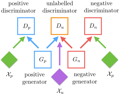
We build our GenPU model upon GAN by leveraging its potentiality in producing realistic data, with the goal of identification of both positive and negative distributions from P and U data. Then, a decision boundary can be made by training standard PN classifier on the generated samples. Figure 1 illustrates the architecture of the proposed framework.
Xu
Figure 1: Our GenPU framework. Dp receives as inputs the real positive examples from Xp and the synthetic positive examples from Gp; Dn receives as inputs the real positive examples from Xp and the synthetic negative examples fromGn; Du receives as inputs real unlabeled examples from Xu, synthetic positive examples from Gp as well as synthetic negative examples from Gn at the same time. Associated with different loss functions, Gp and Gn are designated to generate positive and negative examples, respectively.
In brief, GenPU framework is an analogy to a minimax game comprising of two generators {Gp,Gn} and three discriminators {Dp,Du,Dn}. Guided by the adversarial supervision of {Dp,Du,Dn}, {Gp,Gn} are tasked with synthesizing positive and negative samples that are indistinguishable with the real ones drawn from {pp(x), pn(x)}, respectively. As being their competitive opponents, {Dp,Du,Dn} are devised to play distinct roles in instructing the learning process of {Gp, Gn}.
More formally, the overall GenPU objective function can be decomposed, in views of Gp and Gn, as follows :
where πp and πn corresponding to Gp and Gn are the priors for positive class and negative class, satisfying πp + πn = 1. Here, we assume πp and πn are predetermined and fixed.
The first term linked with Gp in (3) can be further split into two standard GAN components GANGp,Dp and GANGp,Du :
where λp and λu are the weights balancing the relative importance of effects between Dp and Du. In particular, the value functions of GANGp,Dp and GANGp,Du are
On the other hand, the second term linked with Gn in (3) can also be split into GAN components, namely GANGn,Du and GANGn,Dn :
whose weights λu and λn control the trade-off between Du and Dn. GANGn,Du also takes the form of the standard GAN with the value function
The value function of GANGn,Dn is given by
In contrast to the 'zero-sum' loss applied elsewhere, the optimization of GANGn,Dn is given by first maximizing (9) to obtain the optimal D⋆n as
then plugging D⋆n into the value function (9), and finally minimizing -VGn,D⋆n (G,D⋆n ) instead of VGn,D⋆n (G,D⋆n ) to get the optimal G⋆n as
Such modification makes GANGn,Dn different from the standard GAN, and this is reflected by the second term of (7).
Intuitively, (5)-(6) indicate Gp, co-supervised under both Dp and Du, endeavours to minimize the distance between the induced distribution pgp(x) and positive data distribution pp(x), while striving to stay around within the whole data distribution p(x). In fact, Gp tries to deceive both discriminators by simultaneously maximizing Dp's and Du's outputs on fake positive samples. As a result, the loss terms in (5) and (6) jointly guide pgp(x) gradually moves towards and finally settles to pp(x) of p(x).
Equations (8)-(11) suggest Gn, when facing both Du and Dn, struggles to make the induced pgn(x) stay away from pp(x), and also makes its effort to force pgn(x) to lie within p(x). To achieve this, the objective in (11) favors Gn to produce negative examples; this in turn helps Dn to maximize the objective in (10) to separate positive training samples from fake negative samples rather than confusing Dn. Notice that, in the value function (11), Gn is designed to minimize Dn's output instead of maximizing it when feeding Dn with fake negative samples. Consequently, Dn will send uniformly negative feedback to Gn. In this way, the gradient information derived from negative feedback decreases pgn(x) where the positive data region pp(x) is large. In the meantime, the gradient signals fromDu increase pgn(x) outside the positive region but still restricting pgn(x) in the true data distribution p(x). This crucial effect will eventually push pgn(x) away from pp(x) but towards pn(x).
3.3 Theoretical Analysis
Theoretically, suppose all the {Gp,Gn} and {Dp,Du,Dn} have enough capacity. Then the following results show that, at Nash equilibrium point of (3), the minimal JSD between the distributions induced by {Gp,Gn} and the data distributions {pp(x), pn(x)} are achieved, respectively, i.e., pgp(x) = pp(x) and pgn(x) = pn(x). Meanwhile, the JSD between the distribution induced by Gn and data distribution pp(x) is maximized, i.e., pgn(x) almost never overlaps with pp(x).
Proposition 1. Given fixed generators Gp, Gn and known class prior πp, the optimal discriminators Dp, Du and Dn for the objective in equation (3) have the following forms :
and
Proof. Assume that all the discriminators Dp, Du and Dn can be optimized in functional space. Differentiating the objective V(G, D) in (3) w.r.t. Dp, Du and Dn and equating the functional derivatives to zero, we can obtain the optimal D⋆ p , D⋆u and D⋆n as described above.
Theorem 2. Suppose the data distribution p(x) in the standard PU learning setting takes form of p(x) = πppp(x) + πnpn(x), where pp(x) and pn(x) are well-separated. Given the optimal D⋆ p , D⋆u and D⋆n , the minimax optimization problem with the objective function in (3) obtains its optimal solution if
Proof. Substituting the optimal D⋆ p , D⋆u and D⋆n into (3), the objective can be rewritten as follows :
Combining the intermediate terms associated with λu using the fact πp + πn = 1, we reorganize (13) and arrive at
which peaks its minimum if
and for almost every x except for those in a zero measure set
The solution to G = {Gp, Gn} must jointly satisfy the conditions described in (15)-(17), which implies (12) and leads to the minimum objective value of -(πpλp + λu) log(4).
The theorem reveals that approaching to Nash equilibrium is equivalent to jointly minimizing JSD(p‖πppgp + πnpgn) and JSD(pp ‖ pgp) and maximizing JSD(pp ‖ pgn) at the same time, thus exactly capturing pp and pn.
3.4 Connection to Semi-Supervised Classification
The goal of semi-supervised classification is to learn a classifier from positive, negative and unlabeled data. In such context, besides training sets Xp and Xu, a partially labeled negative set Xn is also available, with samples drawn from negative data distribution pn(x).
In fact, the very same architecture of GenPU can be applied to the semi-supervised classification task by just adapting the standard GAN value function to Gn, then the total value function turns out to be
With above formulation, Dn discriminates the negative training samples from the synthetic negative samples produced by Gn. Now Gn intends to fool Dn and Du simultaneously by outputting realistic examples, just like Gp does for Dp and Du. Being attracted by both p(x) and pn(x), the induced distribution pgn(x) gradually approaches to pn(x) and finally recovers the true distribution pn(x) of p(x). Theoretically, it is not hard to show the optimal Gp and Gn, at convergence, give rise to pgp(x) = pp(x) and pgn(x) = pn(x).
4 Experimental Results
We show the efficacy of our framework by conducting experiments on synthetic and real-world images datasets. For real data, the approaches including oracle PN, unbiased PU (UPU) [Du Plessis et al., 2015], non-negative PU (NNPU) [Kiryo et al., 2017] 1 are selected for comparison. Specifically, the Oracle PN means all the training labels are available for all the P and N data, whose performance is just used as a reference for other approaches. For all the methods, the true classprior πp is assumed to be known in advance. Regarding the weights of GenPU, for simplicity, we set λu = 1 and freely tune λp and λn on the validation set via grid search over the range like [... 0.01, 0.02, ... 0.1, 0.2, ..., 1, 2, ....].
4.1 Synthetic Simulation
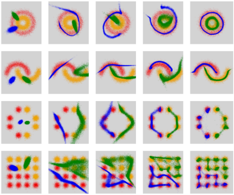
We begin our test with a toy example to visualize the learning behaviors of our GenPU. The training samples are synthesized using concentric circles, Gaussian mixtures and half moons functions with Gaussian noises added to the data (standard deviation is 0.1414). The training set contains 5000 positive and 5000 negative samples, which are then partitioned into 500 positively labelled and 9500 unlabeled samples. We establish the generators with two fully connected hidden layers and the discriminators with one hidden layer. There are 128 ReLU units contained in all hidden layers. The dimensionality of the input latent code is set to 256. Figure 2 depicts the evolution of positive and negative samples produced by GenPU through time. As expected, in all the scenarios, the induced generator distributions successfully converge to the respective true data distributions given limited P data. Notice that the Gaussian mixtures cases demonstrate the capability of our GenPU to learn a distribution with multiple submodes.
4.2 MNIST and USPS Dataset
Next, the evaluation is carried out on MNIST [LeCun et al., 1998] and USPS [LeCun et al., 1990] datasets. For MNIST, we each time select a pair of digits to construct the P and N
1 The software codes for UPU and NNPU are downloaded from https://github.com/kiryor/nnPUlearning
| Operation | Feature Maps | Nonlinearity |
|---|---|---|
| Gp(z),Gn(z): z ∼ N(0, I) fully connected fully connected fully connected Dp(x), Dn(x) fully connected Du(x) fully connected fully connected fully connected leaky relu slope mini-batch size for Xp, Xu learning rate optimizer weight, bias initialization | 100 256 256 256/784 256/784 1 256/784 256 256 1 0.2 50, 100 0.0003 | leaky relu leaky relu tanh sigmoid |
| Adam(0.9, 0.999) 0, 0 | leaky relu leaky relu sigmoid |
sets, each of which consists of 5, 000 training points. The specifics for architecture and hyperparameters are described in Table 1. To be challenging, the results of the most visually similar digit pairs, such as '3' vs '5' and '8' vs '3', are recorded in Table 1. The best accuracies are shown with the number of labeled positive examples Nl ranging from 100 to 1. Obviously, our method outperforms UPU in all the cases. We also observe our GenPU achieves better than or comparable accuracy to NNPU when the number of labeled samples is relatively large (i.e., Nl = 100). However, when the labeled samples are insufficient, for instance Nl = 5 of the '3' vs '5' scenario, the accuracy of GenPU slightly decreases from 0.983 to 0.979, which is in contrast to that of NNPU drops significantly from 0.969 to 0.843. Spectacularly, GenPU still remains highly accurate even if only one labeled sample is provided whereas NNPU fails in this situation.
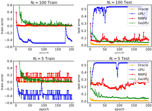
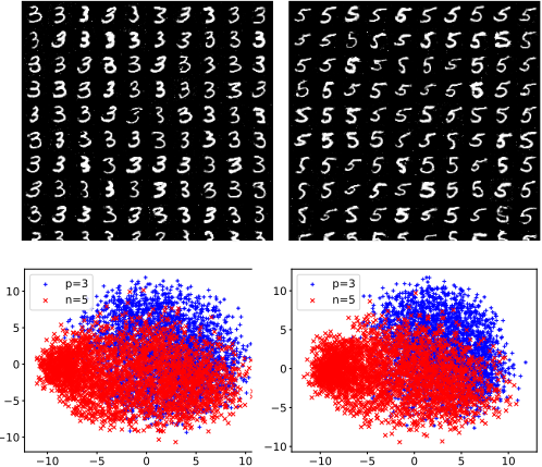
Figure 3 reports the training and test errors of the classifiers for distinct settings of Nl. When Nl is 100, UPU suffers from a serious overfitting to training data, whilst both NNPU and GenPU perform fairly well. As Nl goes small (i.e., 5), NNPU also starts to overfit. It should be mentioned that the negative training curve of UPU (in blue) is because the unbiased risk estimators [Du Plessis et al., 2014; 2015] contain negative loss term which is unbounded from the below. When the classifier becomes very flexible, the risk can be arbitrarily negative [Kiryo et al., 2017]. Additionally, the rather limited Nl cause training processes of both UPU and NNPU behave unstable. In contrast, GenPU avoids overfitting to small training P data by restricting the models of Dp and Dn from being too complex when Nl becomes small (see Table 1). For visualization, Figure 4 demonstrates the generated digits with only one labeled '3', together with the projected distributions induced by Gp and Gn. In Table 3, similar results can be obtained on USPS data.
| MNIST | '3' vs. '5' | '8' vs. '3' | ||||||
|---|---|---|---|---|---|---|---|---|
| Np : Nu | Oracle PN | UPU | NNPU | GenPU | Oracle PN | UPU | NNPU | GenPU |
| 100: 9900 | 0.993 | 0.914 | 0.969 | 0.983 | 0.994 | 0.932 | 0.974 | 0.982 |
| 50: 9950 | 0.993 | 0.854 | 0.966 | 0.982 | 0.994 | 0.873 | 0.965 | 0.979 |
| 10: 9990 | 0.993 | 0.711 | 0.866 | 0.980 | 0.994 | 0.733 | 0.907 | 0.978 |
| 5: 9995 | 0.993 | 0.660 | 0.843 | 0.979 | 0.994 | 0.684 | 0.840 | 0.976 |
| 1: 9999 | 0.993 | 0.557 | 0.563 | 0.976 | 0.994 | 0.550 | 0.573 | 0.972 |
| USPS | '3' vs '5' | '8' vs '3' | ||||
|---|---|---|---|---|---|---|
| Nl : Nu | UPU | NNPU | GenPU | UPU | NNPU | GenPU |
| 50: 1950 | 0.890 | 0.965 | 0.965 | 0.900 | 0.965 | 0.945 |
| 10: 1990 | 0.735 | 0.880 | 0.955 | 0.725 | 0.920 | 0.935 |
| 5: 1995 | 0.670 | 0.830 | 0.950 | 0.630 | 0.865 | 0.925 |
| 1: 1999 | 0.540 | 0.610 | 0.940 | 0.555 | 0.635 | 0.920 |
4.3 Celeb-ADataset
We are also interested in how GenPU performs on the real-life image set. In this set, the data is taken from CelebA dataset [Liu et al., 2015] and resized to 64×64. We aim at classifying female from male using partially labeled male face images.
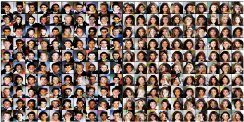
To this end, the first 20, 000 male and 20, 000 female faces in CelebA are chosen as training set and the last 1, 000 faces are used as test set. Then, 2, 000 out of 20, 000 male faces are are randomly selected as positively labeled data. The architectures for generators and discriminators follow the design of the improved WGAN [Gulrajani et al., 2017]. Figure 5 illustrates the generated male and female faces, indicating GenPU is capable of producing visually appealing and diverse images that belong to the correct categories. A deep PN classifier is then trained on the synthetic images and achieves the accuracy of 87.9 which is better than 86.8 of NNPU and 62.5 of UPU.
5 Discussion
One key factor to the success of GenPU relies on the capability of underlying GAN in generating diverse samples with high quality standard. Only in this way, the ideal performance could be achieved by training a flexible classifier on those samples. However, it is widely known that the perfect training of the original GAN is quite challenging. GAN suffers from issues of mode collapse and mode oscillation, especially when high-dimensional data distribution has a large number of output modes. For this reason, the similar issue of the original GAN may happen to our GenPU when a lot of output submodes exist. Since it has empirically been shown that the original GAN equipped with JSD inclines to mimic the mode-seeking process towards convergence. Fortunately, our framework is very flexible in the sense that it can be established by switching to different underlying GAN variants with more effective distance metrics (i.e., integral probability metric (IPG)) other than JSD (or f-divergence). By doing so, the possible issue of the missing modes can be greatly reduced. Another possible solution is to extend single generator Gp (Gn) to multiple generators {Gip }Ii=1 ({Gjn }Ji=1 ) for the positive (negative) class, also by utilizing the parameter sharing scheme to leverage common information and reduce the computational load. Regarding other application domains, one direction of future work is to use GenPU for text classification. However, applying GAN to generating sequential semantically meaningful text is challenging, since GAN has difficulty in directly generating sequences of discrete tokens [Goodfellow et al., 2016]. More sophisticated underlying GANs need to be developed for this purpose.
Acknowledgments
This work was partially supported by JSPS KAKENHI (Grant No. 17K00326), NSFC China (Grant No. 61773129) and JST GREST (Grant No. JPMJCR1784).
@inproceedings{ijcai2018p312,
  title     = {Generative Adversarial Positive-Unlabelled Learning},
  author    = {Hou, Ming and Chaib-draa, Brahim and Li, Chao and Zhao, Qibin},
  booktitle = {Proceedings of the Twenty-Seventh International Joint Conference on
               Artificial Intelligence, {IJCAI-18}},
  publisher = {International Joint Conferences on Artificial Intelligence Organization},
  editor    = {Jérôme Lang},
  pages     = {2255--2261},
  year      = {2018},
  month     = {7},
  note      = {Main track},
  doi       = {10.24963/ijcai.2018/312},
  url       = {https://doi.org/10.24963/ijcai.2018/312},
}
TY - CPAPER TI - Generative Adversarial Positive-Unlabelled Learning AU - Hou, Ming AU - Chaib-draa, Brahim AU - Li, Chao AU - Zhao, Qibin T2 - Proceedings of the Twenty-Seventh International Joint Conference on Artificial Intelligence, IJCAI-18 PB - International Joint Conferences on Artificial Intelligence Organization PY - 2018 SP - 2255 EP - 2261 DO - 10.24963/ijcai.2018/312 UR - https://doi.org/10.24963/ijcai.2018/312 ER -Copied
Machine-readable versions of this paper, for tools and AI agents:





