
Regularizing Deep Neural Networks with an Ensemble-based Decorrelation Method
Proceedings of the Twenty-Seventh International Joint Conference on Artificial Intelligence. Main track. Pages 2177-2183.
https://doi.org/10.24963/ijcai.2018/301
Keywords
- Machine Learning: Neural Networks
- Machine Learning: Machine Learning
- Machine Learning: Deep Learning
Abstract
Although Deep Neural Networks (DNNs) have achieved excellent performance in many tasks, improving the generalization capacity of DNNs still remains a challenge. In this work, we propose a novel regularizer named Ensemble-based Decorrelation Method (EDM), which is motivated by the idea of the ensemble learning to improve generalization capacity of DNNs. EDM can be applied to hidden layers in fully connected neural networks or convolutional neural networks. We treat each hidden layer as an ensemble of several base learners through dividing all the hidden units into several non-overlap groups, and each group will be viewed as a base learner. EDM encourages DNNs to learn more diverse representations by minimizing the covariance between all base learners during the training step. Experimental results on MNIST and CIFAR datasets demonstrate that EDM can effectively reduce the overfitting and improve the generalization capacity of DNNs
- [Abadi et al., 2016] Martín Abadi, Ashish Agarwal, Paul Barham, Eugene Brevdo, Zhifeng Chen, Craig Citro, Greg S Corrado, Andy Davis, Jeffrey Dean, Matthieu Devin, et al. Tensorflow: Large-scale machine learning on heterogeneous distributed systems. arXiv preprint arX- iv:1603.04467, 2016.
- [Bengio and Bergstra, 2009] Yoshua Bengio and James S Bergstra. Slow, decorrelated features for pretraining com- plex cell-like networks. In Advances in neural information processing systems, pages 99-107, 2009.
- [Chandar et al., 2016] Sarath Chandar, Mitesh M Khapra, Hugo Larochelle, and Balaraman Ravindran. Correlation- al neural networks. Neural computation, 2016.
- [Chen et al., 2017] Yunpeng Chen, Xiaojie Jin, Jiashi Feng, and Shuicheng Yan. Training group orthogonal neural net- works with privileged information. arXiv preprint arX- iv:1701.06772, 2017. IJCAI
- [Cheung et al., 2014] Brian Cheung, Jesse A Livezey, Ar- jun K Bansal, and Bruno A Olshausen. Discovering hid- den factors of variation in deep networks. arXiv preprint arXiv:1412.6583, 2014.
- [Cogswell et al., 2015] Michael Cogswell, Faruk Ahmed, Ross Girshick, Larry Zitnick, and Dhruv Batra. Reducing overfitting in deep networks by decorrelating representa- tions. arXiv preprint arXiv:1511.06068, 2015.
- [Geman et al., 1992] Stuart Geman, Elie Bienenstock, and René Doursat. Neural networks and the bias/variance dilemma. Neural computation, 4(1):1-58, 1992.
- [Goodfellow et al., 2016] Ian Goodfellow, Yoshua Bengio, Aaron Courville, and Yoshua Bengio. Deep learning, vol- ume 1. MIT press Cambridge, 2016.
- [Graves et al., 2013] Alex Graves, Abdel-rahman Mohamed, and Geoffrey Hinton. Speech recognition with deep recur- rent neural networks. In Acoustics, speech and signal pro- cessing (icassp), 2013 ieee international conference on, pages 6645-6649. IEEE, 2013.
- [Jozefowicz et al., 2016] Rafal Jozefowicz, Oriol Vinyals, Mike Schuster, Noam Shazeer, and Yonghui Wu. Explor- ing the limits of language modeling. arXiv preprint arX- iv:1602.02410, 2016.
- [Kingma and Ba, 2014] Diederik Kingma and Jimmy Ba. Adam: A method for stochastic optimization. arXiv preprint arXiv:1412.6980, 2014.
- [Krizhevsky et al., 2012] Alex Krizhevsky, Ilya Sutskever, and Geoffrey E Hinton. Imagenet classification with deep convolutional neural networks. In Advances in neural in- formation processing systems, pages 1097-1105, 2012.
- [Krogh and Hertz, 1992] Anders Krogh and John A Hertz. A simple weight decay can improve generalization. In Ad- vances in neural information processing systems, pages 950-957, 1992.
- [Levine et al., 2017] Yoav Levine, David Yakira, Nadav Co- hen, and Amnon Shashua. Deep learning and quantum en- tanglement: Fundamental connections with implications to network design. CoRR, abs/1704.01552, 2017.
- [Rodríguez et al., 2016] Pau Rodríguez, Jordi Gonzàlez, Guillem Cucurull, Josep M Gonfaus, and Xavier Roca. Regularizing cnns with locally constrained decorrelations. arXiv preprint arXiv:1611.01967, 2016.
- [Srivastava et al., 2014] Nitish Srivastava, Geoffrey E Hin- ton, Alex Krizhevsky, Ilya Sutskever, and Ruslan Salakhutdinov. Dropout: a simple way to prevent neural networks from overfitting. Journal of machine learning research, 15(1):1929-1958, 2014.
- [Ueda and Nakano, 1996] Naonori Ueda and Ryohei Nakano. Generalization error of ensemble estimators. In Neural Networks, 1996., IEEE International Conference on, volume 1, pages 90-95. IEEE, 1996.
- [Wan et al., 2013] Li Wan, Matthew Zeiler, Sixin Zhang, Yann Le Cun, and Rob Fergus. Regularization of neural networks using dropconnect. In International Conference on Machine Learning, pages 1058-1066, 2013.
- [Wu et al., 2016] Yonghui Wu, Mike Schuster, Zhifeng Chen, Quoc V Le, Mohammad Norouzi, Wolfgang Macherey, Maxim Krikun, Yuan Cao, Qin Gao, Klaus Macherey, et al. Google's neural machine translation sys- tem: Bridging the gap between human and machine trans- lation. arXiv preprint arXiv:1609.08144, 2016.
- [Wu et al., 2017] Bingzhe Wu, Zhichao Liu, Zhihang Yuan, Guangyu Sun, and Charles Wu. Reducing overfitting in deep convolutional neural networks using redundancy reg- ularizer. In International Conference on Artificial Neural Networks, pages 49-55. Springer, 2017.
- [Xie et al., 2015] Mengjiao Xie, Yuexian Hou, Peng Zhang, Jingfei Li, Wenjie Li, and Dawei Song. Modeling quantum entanglements in quantum language models. 2015. IJCAI
- [Xiong et al., 2016] Wei Xiong, Bo Du, Lefei Zhang, Ruimin Hu, and Dacheng Tao. Regularizing deep con- volutional neural networks with a structured decorrelation constraint. In Data Mining (ICDM), 2016 IEEE 16th In- ternational Conference on, pages 519-528. IEEE, 2016.
- [Zeiler and Fergus, 2014] Matthew D. Zeiler and Rob Fer- gus. Visualizing and understanding convolutional net- works. In In Computer Vision-ECCV 2014, pages 818- 833. Springer, 2014.
- [Zhou, 2012] Zhi-Hua Zhou. Ensemble methods: founda- tions and algorithms. CRC press, 2012.
References were extracted automatically from the PDF and may contain errors.
Full text extracted automatically from the PDF; figures, tables and equations may differ. The PDF is the version of record.
1 Introduction
Deep Neural Networks (DNNs) have achieved great success in many tasks such as image classification [Krizhevsky et al., 2012], machine translation [Wu et al., 2016], language modeling [Jozefowicz et al., 2016] and speech recognition [Graves et al., 2013], which benefits from its powerful learning ability. However, DNNs always bring another problem-overfitting. That is why the large scale datasets are necessary for training DNNs. Therefore, the study on how to avoid overfitting while retaining the strong ability of the DNNs has become important and meaningful. So far, some regularization methods have been proposed to solve this problem, such as Weight Decay [Krogh and Hertz, 1992], Dropout [Srivastava et al., 2014], DropConnect [Wan et al., 2013], etc. These methods improve the generalization capacity of DNNs in different ways. For instance, DropConnect sets a randomly selected subset of weights within the network to zero. Although these methods have been applied to prevent overfitting, they are all in an implicit way.
∗Corresponding author: Yuexian Hou.
Recently, some studies try to explore the reason of the overfitting and find more effective way to avoid overfitting in DNNs [Srivastava et al., 2014; Cogswell et al., 2015; Xiong et al., 2016]. Srivastava et al. [2014] took a further step to explore the nature of the overfitting. They found that for each hidden unit, Dropout could prevent co-adaptation by making the presence of other hidden units unreliable. Inspired by the explanation of Dropout, Cogswell et al. [2015] proposed an effective method named DeCov. They limited the correlation between each units in the same layer by reducing their cross-covariances to improve the generalization performance of the network. However, DeCov tends to influence the learning ability of DNNs because of the breakdown of the correlation between all hidden units. This opinion is proved by our experiments which will be shown in the following sections. Meaningfully, some researchers used quantum-like motivations to explain the representation of the neural networks [Levine et al., 2017]. Actually, the parallel structure of neural networks can be naturally regarded as a classical simulation of general quantum superposition or entanglement states [Xie et al., 2015], which implies that the neural networks is not only a realization of a single statistical-hypothesis but also a realization of multi-statistical-hypothesis. Hence, it is intriguing to analyze neural networks via some point of view of multi-statistical-hypothesis, e.g., ensemble learning.
In this paper, we propose a new regularization method named Ensemble-based Decorrelation Method (EDM). Different from other existing studies, we analyze each hidden layer in DNNs from the perspective of ensemble learning [Zhou, 2012]. Thus, in EDM, the hidden units in the same layer can be divided into several non-overlapping groups, each one will be viewed as a base learner.
The goal of EDM is the same as ensemble learning, both of which aim to improve the learning ability of each base learner and increase diversity between different base learners to get diverse features simultaneously. Aiming to improve learning ability, we try to obtain stronger base learners through assigning several units in one group instead of splitting them one by one. For increasing diversity, we limit the correlation between different groups, so as to decrease the generalization error and enhance the generalization capacity of the DNNs according to the bias-variance-covariance decomposition [Ueda and Nakano, 1996].
Besides fully connected neural network, EDM can also be applied to the pooling layers in Convolutional Neural Network (CNN). In the pooling layer, the only difference is that a pooled feature map is considered as a base learner. In this paper, we adopt covariance between base learners as the measurement of correlation, and put it to the loss function of the network as a regularization term.
The experimental results show that comparing with other existing regularization methods, EDM can achieve better performance and effectively improve the generalization capacity of DNNs. Further, the correlation between hidden units are demonstrated as a crucial factor for reducing the overfitting in DNNs.
2 Ensemble-based DecorrelationMethod
This section introduces the Ensemble-based Decorrelation Method (EDM), a regularizer that aims to decrease correlation between hidden units in hidden layer so as to reduce the overfitting in DNNs.
2.1 Theoretical Motivation
It is well known that the bias-variance decomposition is an important theory tool for explaining the generalization performance of the learning algorithms [Geman et al., 1992]. It divides the generalization error of a learner into three parts, i.e., bias, variance and noise. Since the noise is difficult to estimate, it is usually subsumed into the bias term. Let yD denote the target on the dataset D and fD denote the predicted output of the learner on the dataset D, the error function can be defined as:
where the bias and variance of the learner fD are defined as:
Based on this, Ueda et al. [1996] proposed a bias-variancecovariance decomposition for an ensemble of M base learners {f 1D , f 2D , ..., f M D }, which is defined as:
where
where FD = 1M ∑Mm=1 f m D . The formula (4) shows that the generalization error depends heavily on the covariance term, which models the correlation between different base learners. The smaller the covariance, the better the ensemble [Zhou, 2012].
Motivated by this theory, reducing the covariance termmay be a compelling idea for enhancing the performance of the DNNs if we regard the hidden layer as an ensemble of several base learners.
2.2 EDM in Fully Connected Neural Network
We first apply EDM on the hidden layer of a fully connected neural network, whose input is a batch of N samples. One can denote the correlation using the covariance, since the lower covariance of two variables usually means a lower linear correlation. Hence, we calculate the covariance matrix of the hidden activations on a batch of samples to keep the correlation between hidden units as lower as possible.
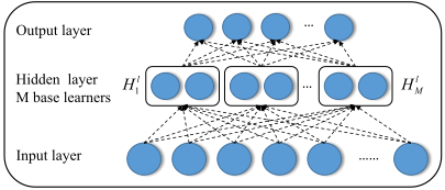
Throughout the paper, let Dl denote the number of units in the l-th layer, W l ∈ RDl-1×Dl denote the weights matrix from the (l - 1)-th to the l-th layer, the activation of the lth hidden layer is Hl ∈ RN×Dl . As the analysis mentioned in introduction, we evenly divide the units into M nonoverlapping groups and regard them as M base learners. Therefore each base learner has k = Dl /M units. The m-th base learner is represented as Hlm ∈ RN×k , which contains the activations of units from the ((m - 1) × k + 1)-th to the (m× k)-th. EDM can encourage the network to learn more diverse and non-redundant representations and improve the generalization capacity of the network by reducing the correlation between different base learners as much as possible. The structure of the ensemble-based decorrelation neural network is showed in Figure 1.
We use GCovpq to represent the covariance between the p-th and q-th base learner, then it can be written as:
where Hl-1 denotes the activation of the (l - 1)-th hidden layer. For facilitating the calculation of covariance, let gn p denote the n-th activation of the p-th base learner, and µp = 1N ∑Nn=1 gn p is the sample mean of the p-th learner's activation over the batch. The covariance is limited to be small by minimizing the Frobenius norm of GCov. Since the diagonal of GCov is the self-correlation coefficients, we can subtract this term from the matrix norm to calculate a final penalty term as follows.
where ‖ · ‖F is the Frobenius norm, and diag(·) operator extracts the main diagonal elements of a matrix into a vector. With the correlation between different base learners being reduced, the generalization performance of neural network can be improved by punishing the GCovloss term. The total loss of the fully connected neural network regularized with EDM method can be formulated as:
where Eloss is the cross entropy loss of the network without any regularizers, Tloss denotes the total loss, λ is the hyperparameter, and λ ≥ 0.
To demonstrate the validity of the total loss, we consider its gradient with respect to the specific i-th activation for a specific sample d:
From these formulas, the GCovloss is consistent with the L2 regularizer, because they both prevent weight from becoming too large and the network from getting overfitting. Particularly, from the formula (14), the weights could be updated by backpropagation according to the covariance term so as to decrease the redundant information between hidden units.
2.3 EDM in Convolutional Neural Network
In theory, we could decorrelate the features obtained by convolutional layers. But the huge amount of parameters implied in convolution layers will bring terrible computation cost. In this section, we mainly consider learning more diverse feature representations of pooling layer in CNN to avoid features being correlated and reduce overfitting as much as possible. Neither a collection of pooled feature maps nor each feature in the pooled feature map is seen as the base learner, we regard a pooled feature map as a base learner for two reasons: (1) a pooled feature map has enough ability of extracting useful features from the image [Goodfellow et al., 2016]; (2) if we regard each feature as a base learner, it will destroy the intrinsic structure and learning ability of the pooling layer. Moreover, minimizing the correlation of all the base learners will generate a very large computation complexity, so we should encourage different pooled feature maps to be diverse instead. The structure of the ensemble-based decorrelation on pooling layer in CNN is showed in Figure 2.
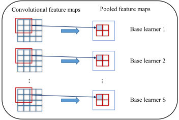
Let i and j index different maps (i.e., the i-th and j-th base learners) in the specific pooling layer. H, W are the height and width of the map respectively. We calculate the covariance between the i-th learner and the j-th learner:
where e(h,w) i is the value in the i-th pooled feature map and mi is the mean value of the i-th map on the batch.
Finally, the penalty loss PoCorloss is obtained and added to the cross entropy loss of the CNN:
where γ is the hyper-parameter, and γ ≥ 0. If we do not apply the EDM method on the fully connected layer in CNN, then set λ = 0.
3 Experiments
3.1 Experiment on Fully Connected Neural Network
Dataset: In order to validate the effectiveness of EDM, we conduct experiments on MNIST dataset, which has a training set of 60000 samples and a test set of 10000 samples. In this work, instead of using the original MNIST dataset, we use a new MNIST dataset with Gaussian noise added. Figure 4 shows a few samples.
Experimental Settings: Since the goal is to evaluate the performance of different regularization method and demonstrate the role of the correlation between hidden units, we choose to set a relatively small network structure. For the Gaussian noise added dataset, we use a 3 layer fully connected neural network, i.e., 1 input layer, 1 output layer and 1 hidden layer with 300 hidden units. We use the Adam [Kingma and Ba, 2014] algorithm to train the network, and the initial learning rate is 0.001. The batch size is 100, and the number of hidden units in each base learner (i.e., the value of k) is 20. The experiments are implemented by Tensorflow [Abadi et al., 2016].

Regularizer Comparisons: Table 1 shows the classification results of different regularization methods on the MNIST dataset. From Table 1, we can observe that EDM gets the best results on the term of test accuracy and achieves the minimum train-test accuracy gap, we also employ t-test to perform the significance test in this experiment, both of which demonstrate that our proposed EDM is effective.
The most noteworthy is that DeCov method achieves the worst performance both on the term of test accuracy and the train-test accuracy gap and the underfitting even occurs on training set. This shows that in a small scale network structure, DeCov decorrelates too many features between hidden units, which may destroy the internal structure of the hidden layer and weaken the learning ability of the network.
Different from DeCov, EDM only reduces the correlation between different base learners, which increases the diversity of the ensemble. To some extent, EDM allows the units to cooperate and retains the stronger learning ability of each base learner. Thus, as the experimental results show, EDM
| Methods | Train | Test | Train-Test |
|---|---|---|---|
| None | 94.80 | 81.85 | 12.95 |
| Dropout | 91.90 | 79.55 | 12.35 |
| DeCov | 73.81 | 58.87 | 14.94 |
| EDM | 91.89 | 84.47† | 7.42† |
achieves the best performance both on the term of test accuracy and train-test accuracy gap.
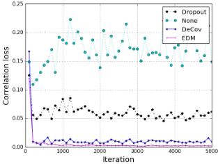
Figure 3 shows the performance of different regularization methods on decreasing correlation loss of hidden layer. From this figure, it is obvious that the correlation loss grows steadily with the None method, indicating that the hidden units are easier to be co-adapted and redundant during training. Other regularization methods significantly reduce the correlation loss of the hidden units. Especially, EDM achieves the best performance.
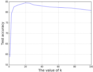
In order to take a further step on analyzing the structure of the hidden layer, we present the accuracy according to the different number of hidden units in each base layer, i.e., the value of k. From Figure 5, we can see that the classification accuracy begins to rise obviously but then shows a downward trend as the value of k increases.
Discussion: These experimental results are consistent with the theory of ensemble learning. For improving the performance of the ensemble, each base learner needs a strong learning ability; moreover, the diversity between all base learners needs to be increased. The changes of k reflects the changes of the learning ability of each base learner. Thus, in order to improve the learning ability of each base learner, the value of k should be controlled in a reasonable range. If k is very small, the learning ability of each base learner will be affected; while if k is too large, there could be only a few base learners and the performance of the ensemble could be poor. Considering a more extreme case, i.e., the value of k is equal to the number of units in hidden layer, it means that there is only one base learner in the ensemble. Obviously its classification performance is generally worse than the other ensembles with more base learners.
All these results indicate that the proposed EDM is more effective than other conventional regularization methods both experimentally and theoretically.
3.2 Experiments on Convolutional Neural Network
Datasets: The CIFAR-10 dataset consists of 60000 images with 32×32 in 10 classes. It has been split into 50000 training images and 10000 test images. The CIFAR-100 dataset is just like the CIFAR-10 dataset, expect that it has 100 classes containing 600 images each. There are 500 training images and 100 testing images per class.
| Methods | CIFAR-10 | CIFAR-100 | ||||
|---|---|---|---|---|---|---|
| Train | Test | Train-Test | Train | Test | Train-Test | |
| None∗ | 100 | 74.35 | 25.65 | 98.70 | 38.83 | 59.87 |
| Dropout∗ | 96.54 | 75.60 | 20.94 | 84.94 | 41.14 | 43.80 |
| DeCov∗ | 88.62 | 75.98 | 12.64 | 73.36 | 40.71 | 32.65 |
| EDM on pool 1 | 91.91 | 77.04 | 14.87 | 72.26 | 42.08 | 30.18 |
| EDM on pool 2 | 91.42 | 77.49 | 13.93 | 73.36 | 42.96 | 30.40 |
| EDM on fully connected layer | 90.48 | 76.64 | 13.84 | 71.06 | 40.93 | 30.13 |
| EDM on fully + pool 1 | 88.63 | 77.02 | 11.61 | 73.75 | 42.60 | 31.15 |
| EDM on fully + pool 2 | 91.64 | 76.99 | 14.65 | 71.80 | 43.39† | 28.41† |
Experimental Settings: Since the goal of our work is to evaluate the effectiveness of EDM on pooling layer. We choose to use a simple CNN architecture, i.e., 3 convolutional layers and each convolutional layers is followed by a pooling layer, a fully connected layer and a softmax layer. The only difference of the network between CIFAR-10 and CIFAR-100 is that the later uses 100 hidden units on softmax layer instead of 10. We use Adam algorithm [Abadi et al., 2016] to train these networks, the initial learning rate is 0.001 and the batch size is 128.
Regularizer Comparisons: Moreover, since Dropout and DeCov methods are usually used to the fully connected layer, we also apply EDM method on the fully connected layer to be compared with other regularization methods more fairly. Table 2 shows the performance comparison of EDM with other regularization methods on the CIFAR-10 and CIFAR100 datasets respectively. Method names with ∗ indicate that they are reimplemented by ourselves.
According to the data from Table 2, on CIFAR-10 dataset, we can observe that EDM performs better, and it achieves an improvement of 3.14 points compared with the None method on the term of test accuracy. Moreover, we can observe that DeCov also achieves significant performance on the term of test accuracy and train-test accuracy gap compared with Dropout. Especially, when EDM is applied on the first and second pooling layers (denoted as pool 1 and pool 2), DeCov performs better than EDM on train-test accuracy gap. However, when we apply the EDM both on the fully connected layer and the first pooling layer, EDM performs much better than DeCov both on test accuracy and train-test accuracy gap. This is because DeCov limits all the correlation between hidden units, which will have a negative influence on the network's learning ability.
On CIFAR-100 dataset, EDM achieves more significant results. There is a 4.56 points promotion on the term of test accuracy, which demonstrates the effectiveness of our EDM method on reducing overfitting in DNNs. Compared with DeCov, EDM has a 2.68 points promotion on the term of test accuracy, and it also obtains the best performance on traintest accuracy gap. When the EDM is applied on the fully connected layer in CNN, the test accuracy decreases slightly compared with Dropout but it achieves the best performance on train-test accuracy gap, which further demonstrates the superiority of EDM.
Specially, analyzing how our EDM behaves on CIFAR-10 and CIFAR-100 datasets, it is obvious that the performance of EDM on the pooling layer is more significant than on the fully connected layer. On CIFAR-100 dataset, when applying EDM on the second pooling layer, it even achieves a 2.03 points promotion on the term of test accuracy than applying EDM on the fully connected layer. Therefore, in order to evaluate the performance of EDM in pooling layer more efficiently, we further explore the structure of the pooling layer. We try to divide the pooled feature maps into several non-overlapping groups, and consider each group as a base learner. The value of k is the number of pooled feature maps in each group.
From Table 3 and Table 4, on the CIFAR-10 dataset, we can find that EDM achieves the best performance on the first and second pooling layer when k = 1. However, it is noteworthy that on the CIFAR-100 dataset, although k = 4 and k = 2 achieve the best train-test accuracy gap on the first and second pooling layer respectively, their performance on the test set is much worse. This is because when the pooled feature maps are divided into several nonoverlapping groups, the underfitting may occur on the training set.
Discussion: According to the experimental results, there are two interesting phenomena on pooling layer that are worth discussing, i.e., the advantage of EDM on pooling layer than on fully connected layer and the effectiveness of EDM without grouping the pooled feature maps.
For the former:
(1) In contrast to a single hidden unit of a fully connected hidden layer, a single pooled feature map contains more parameters. Some research on CNN [Zeiler and Fergus, 2014; Goodfellow et al., 2016] further show the learning ability of the pooled feature maps. Accordingly, a single pooled feature map can be viewed as a stronger base learner.
(2) In CNN, take image recognition for instance, the function of the convolution kernel is to extract features of the image from a certain perspective. The greater the difference between the features extracted by different convolution kernels, the more diverse feature can be extracted from the image. Consequently, for the pooling layer, the less redundant information between pooled feature maps, the more generalization performance of the network can be improved.
| The value of k | CIFAR-10 | CIFAR-100 | ||||
|---|---|---|---|---|---|---|
| Train | Test | Train-Test | Train | Test | Train-Test | |
| k=1 | 91.91 | 77.04 | 14.87 | 72.26 | 42.08 | 30.18 |
| k=2 | 93.23 | 75.77 | 17.46 | 65.55 | 40.94 | 24.61 |
| k=4 | 95.38 | 76.86 | 18.52 | 60.94 | 40.56 | 20.38 |
| k=8 | 93.68 | 76.27 | 17.41 | 62.27 | 40.71 | 21.56 |
| The value of k | CIFAR-10 | CIFAR-100 | ||||
|---|---|---|---|---|---|---|
| Train | Test | Train-Test | Train | Test | Train-Test | |
| k=1 | 91.42 | 77.49 | 13.93 | 73.36 | 42.96 | 30.40 |
| k=2 | 92.23 | 76.69 | 15.54 | 60.98 | 41.12 | 19.86 |
| k=4 | 94.68 | 76.47 | 18.21 | 63.44 | 41.04 | 22.40 |
| k=8 | 93.28 | 76.71 | 16.57 | 63.28 | 40.81 | 22.47 |
For the latter, based on the above two reasons, we can conclude that it is not suitable for grouping the pooled feature maps in pooling layer.
One feature map as a base learner: We regard each pooled feature map as a base learner so that the covariance loss would promote different pooled feature maps to extract different features as much as possible. Then the pooling layer can be regarded as an ensemble of several decorrelated base learners.
A group of feature maps as a base learner: When different convolution kernels extract features in one specific region of the image, the extracted features are likely to be redundant. In this case, if we only reduce the correlation between different groups, some correlation within a group will be neglected. Therefore, underfitting is more prone to occur on the training set, and the generalization performance of the network will not be enhanced as expected.
4 RelatedWork
Improving the generalization performance of deep neural networks has received an increasing attention recently. From the literature, two different regularization techniques can be defined.
The first one focuses on decreasing the correlation between hidden units [Bengio and Bergstra, 2009; Cheung et al., 2014; Chandar et al., 2016]. Bergstra et al. [2009] introduced a new type of activation function, which aimed at learning decorrelated representations for pre-training image models. However, in this work, decorrelation was used for initialization unlike our EDMmethod, used for reducing overfitting.
The second type of regularization methods are mainly focused on decorrelating the weights or convolutional functions [Rodr´ıguez et al., 2016; Chen et al., 2017; Wu et al., 2017]. For instance, Rodr´ıguez et al. [2016] proposed OrthoReg method, a regularizer that concentrated on weights correlation rather than activation independence and utilized the cosine similarity between weight features to express their relevance. OrthoReg allowed the regularizer to reach higher decorrelation bounds to reduce the overfitting in CNN. In addition, Chen et al. [2017] proposed GoCNN method, which encouraged learning more diverse representations with each layer by exploring provided privileged information.
However, these methods do not give an explicit explanation for improving the generalization capacity of the CNN, and neglect the redundant information in feature maps. Our proposed EDM method is applied on feature maps of pooling layers in CNN. Unlike grouping the convolutional functions in GoCNN, we analyze the structure of the pooling layer from the perspective of the ensemble learning as described in Section 2.
5 Conclusion
Overfitting is an important factor that affects the performance of the deep neural networks. In this paper, we propose an effective regularizer to avoid overfitting called Ensemble-based Decorrelation Method (EDM), which is motivated by the idea of ensemble learning. Experimental results demonstrate that our method can avoid overfitting and enhance the generalization capacity effectively both in fully connected neural network and convolutional neural network. No matter how challenging the dataset is, our method also can achieve a better performance compared to other existing regularization methods.
Although our method performs better, there are still some deficiencies, such as how to more precisely represent the diversity of units and define the correlation between different base learners are still worth studying.
Acknowledgments
This work is funded in part by the national key research and development program of China (2017YFE0111900), the Key Project of Tianjin Natural Science Foundation (15JCZDJC31100), the National Natural Science Foundation of China (Key Program, U1636203), the National Natural Science Foundation of China (U1736103) and MSCA-ITN-ETN - European Training Networks Project (QUARTZ).
@inproceedings{ijcai2018p301,
  title     = {Regularizing Deep Neural Networks with an Ensemble-based Decorrelation Method},
  author    = {Gu, Shuqin and Hou, Yuexian and Zhang, Lipeng and Zhang, Yazhou},
  booktitle = {Proceedings of the Twenty-Seventh International Joint Conference on
               Artificial Intelligence, {IJCAI-18}},
  publisher = {International Joint Conferences on Artificial Intelligence Organization},
  editor    = {Jérôme Lang},
  pages     = {2177--2183},
  year      = {2018},
  month     = {7},
  note      = {Main track},
  doi       = {10.24963/ijcai.2018/301},
  url       = {https://doi.org/10.24963/ijcai.2018/301},
}
TY - CPAPER TI - Regularizing Deep Neural Networks with an Ensemble-based Decorrelation Method AU - Gu, Shuqin AU - Hou, Yuexian AU - Zhang, Lipeng AU - Zhang, Yazhou T2 - Proceedings of the Twenty-Seventh International Joint Conference on Artificial Intelligence, IJCAI-18 PB - International Joint Conferences on Artificial Intelligence Organization PY - 2018 SP - 2177 EP - 2183 DO - 10.24963/ijcai.2018/301 UR - https://doi.org/10.24963/ijcai.2018/301 ER -Copied
Machine-readable versions of this paper, for tools and AI agents:





