
Cuckoo Feature Hashing: Dynamic Weight Sharing for Sparse Analytics
Proceedings of the Twenty-Seventh International Joint Conference on Artificial Intelligence. Main track. Pages 2135-2141.
https://doi.org/10.24963/ijcai.2018/295
Keywords
- Machine Learning: Feature Selection ; Learning Sparse Models
- Machine Learning: Dimensionality Reduction and Manifold Learning
- Computer Vision: Big Data and Large Scale Methods
Abstract
Feature hashing is widely used to process large scale sparse features for learning of predictive models. Collisions inherently happen in the hashing process and hurt the model performance. In this paper, we develop a feature hashing scheme called Cuckoo Feature Hashing(CCFH) based on the principle behind Cuckoo hashing, a hashing scheme designed to resolve collisions. By providing multiple possible hash locations for each feature, CCFH prevents the collisions between predictive features by dynamically hashing them into alternative locations during model training. Experimental results on prediction tasks with hundred-millions of features demonstrate that CCFH can achieve the same level of performance by using only 15%-25% parameters compared with conventional feature hashing.
- [Attenberg et al., 2009] Josh Attenberg, Kilian Weinberger, Anirban Dasgupta, Alex Smola, and Martin Zinkevich. Collaborative email-spam filtering with the hashing trick. In CEAS, 2009.
- [Caragea et al., 2012] Cornelia Caragea, Adrian Silvescu, and Prasenjit Mitra. Protein sequence classification using feature hashing. Proteome science, 2012.
- [Chen et al., 2015] Wenlin Chen, James T Wilson, Stephen Tyree, Kilian Q Weinberger, and Yixin Chen. Compress- ing neural networks with the hashing trick. In ICML, 2015.
- [Cunningham and Ghahramani, 2015] John P Cunningham and Zoubin Ghahramani. Linear dimensionality reduction: survey, insights, and generalizations. JMLR, 2015.
- [He and Chua, 2017] Xiangnan He and Tat-Seng Chua. Neu- ral factorization machines for sparse predictive analytics. In SIGIR, 2017.
- [He and Niyogi, 2004] Xiaofei He and Partha Niyogi. Lo- cality preserving projections. In NIPS, 2004.
- [Ihaka and Gentleman, 1996] Ross Ihaka and Robert Gentle- man. R: a language for data analysis and graphics. JCGS, 1996.
- [Jang et al., 2011] Jiyong Jang, David Brumley, and Shobha Venkataraman. Bitshred: feature hashing malware for scalable triage and semantic analysis. In CCS, 2011.
- [Juan et al., 2016] Yuchin Juan, Yong Zhuang, Wei-Sheng Chin, and Chih-Jen Lin. Field-aware factorization ma- chines for ctr prediction. In RecSys, 2016.
- [Kingma and Ba, 2014] Diederik P Kingma and Jimmy Ba. Adam: A method for stochastic optimization. arXiv preprint arXiv:1412.6980, 2014.
- [Kutzelnigg, 2006] Reinhard Kutzelnigg. Bipartite random graphs and cuckoo hashing. In Fourth Colloquium on Mathematics and Computer Science Algorithms, Trees, Combinatorics and Probabilities. Discrete Mathematics and Theoretical Computer Science, 2006.
- [Ma et al., 2009] Justin Ma, Lawrence K Saul, Stefan Sav- age, and Geoffrey M Voelker. Identifying suspicious urls: an application of large-scale online learning. In ICML, 2009.
- [Mahout, 2012] Apache Mahout. Scalable machine learning and data mining, 2012.
- [Meng et al., 2016] Xiangrui Meng, Joseph Bradley, Burak Yavuz, Evan Sparks, Shivaram Venkataraman, Davies Liu, Jeremy Freeman, DB Tsai, Manish Amde, and Sean Owen. Mllib: Machine learning in apache spark. JMLR, 2016.
- [Mika et al., 1999] Sebastian Mika, Gunnar Ratsch, Jason Weston, Bernhard Scholkopf, and Klaus-Robert Mullers. Fisher discriminant analysis with kernels. In Neural Net- works for Signal Processing, 1999.
- [Pagh and Rodler, 2001] Rasmus Pagh and Flemming Friche Rodler. Cuckoo hashing. Springer, 2001.
- [Pedregosa et al., 2011] Fabian Pedregosa, Gaël Varoquaux, Alexandre Gramfort, Vincent Michel, Bertrand Thirion, Olivier Grisel, Mathieu Blondel, Peter Prettenhofer, Ron Weiss, Vincent Dubourg, et al. Scikit-learn: Machine learning in python. JMLR, 2011.
- [Richardson et al., 2007] Matthew Richardson, Ewa Domi- nowska, and Robert Ragno. Predicting clicks: estimating the click-through rate for new ads. In WWW, 2007.
- [Shan et al., 2016] Ying Shan, T Ryan Hoens, Jian Jiao, Hai- jing Wang, Dong Yu, and JC Mao. Deep crossing: Web- scale modeling without manually crafted combinatorial features. In SIGKDD, 2016.
- [Shepitsen et al., 2008] Andriy Shepitsen, Jonathan Gem- mell, Bamshad Mobasher, and Robin Burke. Personalized recommendation in social tagging systems using hierarchi- cal clustering. In RecSys, 2008.
- [Shi et al., 2009] Qinfeng Shi, James Petterson, Gideon Dror, John Langford, Alex Smola, and SVN Vish- wanathan. Hash kernels for structured data. JMLR, 2009.
- [Song et al., 2011] Jingkuan Song, Yi Yang, Zi Huang, Heng Tao Shen, and Richang Hong. Multiple feature hash- ing for real-time large scale near-duplicate video retrieval. In ACM MM, 2011.
- [Wall et al., 2003] Michael E Wall, Andreas Rechtsteiner, and Luis M Rocha. Singular value decomposition and principal component analysis. In A practical approach to microarray data analysis. 2003.
- [Weinberger et al., 2009] Kilian Weinberger, Anirban Das- gupta, John Langford, Alex Smola, and Josh Attenberg. Feature hashing for large scale multitask learning. In ICML, 2009.
- [Yan et al., 2007] Shuicheng Yan, Dong Xu, Benyu Zhang, Hong-Jiang Zhang, Qiang Yang, and Stephen Lin. Graph embedding and extensions: A general framework for di- mensionality reduction. TPAMI, 2007.
- [Zaharia et al., 2010] Matei Zaharia, Mosharaf Chowdhury, Michael J Franklin, Scott Shenker, and Ion Stoica. Spark: Cluster computing with working sets. HotCloud, 2010.
- [Zhou et al., 2015] Li Zhou, David G Andersen, Mu Li, and Alexander J Smola. Cuckoo linear algebra. In SIGKDD, 2015.
References were extracted automatically from the PDF and may contain errors.
Full text extracted automatically from the PDF; figures, tables and equations may differ. The PDF is the version of record.
1 Introduction
Many industry-scale machine learning applications are conducted on sparse feature datasets, some of which contain more than hundreds of millions of features in a thousandbillion dimensional space. Examples include personalized spam filtering [Attenberg et al., 2009], advertisement click through rate (CTR) prediction [Richardson et al., 2007], recommendation system [Shepitsen et al., 2008], DNA analysis [Caragea et al., 2012], and etc. Feature hashing [Shi et al., 2009; Weinberger et al., 2009] (i.e. hash kernel), widely used to process sparse features in high-dimensional space due to its strength in time and space efficiency, has been accepted as a conventional method for sparse feature processing in most ML libraries and platforms, such as scikit-learn [Pedregosa et al., 2011], Mahout [Mahout, 2012], Spark [Zaharia et al., 2010; Meng et al., 2016] and R [Ihaka and Gentleman, 1996]. By applying a hash function to directly map the features to corresponding data buckets, feature hashing efficiently processes sparse features without relying on an index to look up the feature values (i.e., weights). Feature hashing also reduces the number of feature dimensions, as features are randomly grouped into hash buckets, where the co-located features share the same weight.
While existing feature hashing schemes [Weinberger et al., 2009] are shown to be efficient, the resultant model performance may suffer when the predictive features with different expected weights are hashed into the same bucket, and as a result share the same parameter weight. Moreover, weight sharing may hurt the sparsity of the model, since non-predictive features hashed together with predictive features also receive non-zero weights instead of zero. Although multiple hashing is proposed to help reducing the inaccuracy caused by collisions, it increases the variance of model and further hurts the model sparsity. The increase of variance and loss of sparsity may result in over-fitting and worse performance when dealing with unseen new features [Weinberger et al., 2009].
In this paper, we treat feature hashing as a problem of dynamic weight sharing and devise a new feature hashing scheme, namely Cuckoo Feature Hashing (CCFH), to determine the locations for predictive features during training, while avoiding most collisions. As the name suggests, CCFH exploits the idea of Cuckoo hashing [Pagh and Rodler, 2001] to use two hash functions to provide two alternative locations for each feature. When data collision occurs, the data in the occupied entry can be moved to its alternative location. Any key already residing in this location is then displaced to its alternative location. This collision resolution process continues until a vacant position is found. It is guaranteed that almost all collisions can be resolved when the load factor of hash table is smaller than 0.5, and each collision can be resolved in amortized constant operations. Thus, it is able to dynamically and flexibly "adjust" the hash functions to resolve collisions among predictive features.
The novelty of CCFH lies in leveraging a set of indicators in the process of model training to decide the weight of each feature based on its two possible locations. In CCFH, these indicators are treated as parameters, hashed for model compressing, and learnt from simple gradient descent based algorithms. To realize the aforementioned ideas for feature hashing in CCFH, several technical challenges arise. First, there is no key but only value stored in the hash table. A protocol needs to be designed to find for each feature which of the two possible locations stores its actual weight. Second, Cuckoo hashing resolves collisions via its recurrent displacing operations, while it is not clear how such collision resolving scheme can be realized during model training. Finally, CCFH needs to preserve model sparsity by locating most nonpredictive features at zero weight.
In summary, CCFH exhibits several major advantages: (1) its hashing structure is adaptive during model training to minimize the loss; (2) it achieves much smaller hash table when guaranteeing the same level of model performance; and (3) its resolves collisions between predictive features as well as preserves the model sparsity by assign zero weight to nonpredictive features.
Experimental results on public benchmark CTR datasets Avazu and malicious URL detection dataset show that compared with feature hashing and multiple hashing, CCFH can further reduce the number of parameters by around 4x to 8x to achieve the same model performance.
2 Preliminaries and RelatedWorks
2.1 Feature Hashing
Feature hashing (i.e. hashing trick, hash kernel) [Shi et al., 2009] has been widely used as a dimension reduction technique for sparse features [Song et al., 2011; Jang et al., 2011; Caragea et al., 2012]. Given a vector in a d-dimensional space x ∈ Rd , a mapping function φ : Rd → Rk is learned to project it into k-dimensional space Rk where k ≪ d. We denote Rd as the original space and Rk as the hashed space. The sparse features x are projected to a low dimensional vector φ(x) via a map function
where h(·) : {1, ..., d} → {1, ..., k} defines the one-toone dimension mapping between the two spaces and s(·) : {1, ..., d} → {±1} is a random signal function. It can be shown that function φ preserves the unbiased expectation of inner product operations between the feature input x and weight w, i.e.
since the signal function s(·) ensures that for i ̸= j:
Therefore, for all learning models, the dot-product operation wT x in the original space Rd can be approximated by the dotproduct φ(w)T φ(x) in the hashed space Rk . Feature hashing leads to large memory savings and significant model size reduction, because 1) it can operate directly on the sparse input features (e.g. n-grams, frequent patterns, features generated from Cartesian product etc.) and avoids the use of a dictionary to translate features into vectors; 2) the parameter vector of a learning model resides in the much smaller dimensional hashed space Rk instead of the original space Rd .
To achieve dimensionality reduction and a smaller parameter size k, where k ≪ d, there naturally exist considerable amounts of collisions as multiple features may be hashed into the same dimension. The rationale of applying feature hashing is that the number of predictive features is inherently small compared with the whole feature set and can be represented using the hashed space Rd , i.e. the predictive features are sparse. Therefore, the weight associated with each hashed location is primarily dependent on the most predictive feature in it. The collisions between predictive features may cause severe performance degradation.
Multiple hashing [Weinberger et al., 2009] is the current solution for resolving hash collisions. By using c hashing functions, the mapping function φ(·) is calculated via:
The collisions in multiple hashing are increased by c times while the magnitude of error introduced by each collision is reduced by 1/c. As shown in [Weinberger et al., 2009], multiple hashing also faces three major limitations: 1) reducing the standard variance error ||φ(w)T φ(x) - wT x||2 by c-1/2 with c times computational cost. 2) the error is reduced by sacrificing model sparsity, which contradicts the rationale of applying feature hashing. 3) increases the variance of model and tends to overfit.
2.2 Feature Engineering
There are lots of feature engineering solutions such as factorization machine [Juan et al., 2016; He and Chua, 2017] and feature combination mining [Shan et al., 2016]. These methods are also frequently used for recommendation system and Ads CTR prediction. Feature engineering is actually a dual problem of feature hashing. The reason of applying feature engineering is to make input samples linear-separable by creating new features. In contrast, feature hashing considers the cases where input samples are already linear-separable and there is a need to reduce the problem size (i.e. dimensionality reduction). In many cases, feature engineering and feature hashing can be sequentially applied to introduce a linearseparable feature set of proper size.
2.3 Dimensionality Reduction
Dimensionality reduction methods [Yan et al., 2007; Cunningham and Ghahramani, 2015] aim to find a reduction mapping φ : Rd → Rk to minimize certain loss function. For all linear dimensionality reduction methods, the mapping function φ can be described using a projection matrix P, i.e. φ(x) = Px. For example, principle component analysis (PCA) [Wall et al., 2003] for a given dataset X = [x1, ..., xn] aims at preserving the inner-product operations for all data pairs by minimizing ||(PX)T PX-XT X||2 . For least discriminant analysis (LDA) [Mika et al., 1999] and locality preserving projection (LPP) [He and Niyogi, 2004], only labelspecific and neighborhood pairs are preserved respectively. For most of these methods the mapping P is learnt from data distribution or predictive task. While all these methods may achieve superior performance compared with feature hashing in their applied scenario, the computational complexity of these methods are at least O(kd) (using SGD to compute SVD, or O(k2d) for exact optimization), and the space complexity for P is also O(kd). For large-scale analytics tasks such as advertisement click-through rate (CTR) prediction and personalized spam filtering [Richardson et al., 2007; Attenberg et al., 2009; Ma et al., 2009], d could reach hundred-million or billion level, and k could also reach million level. These dimensionality reduction techniques are not applicable to large scale analytics tasks targeted in this paper.
Feature hashing can be viewed as a very efficient dimensionality reduction method. Unlike most dimensionality reduction where the mapping function φ is carefully learnt, φ in feature hashing is a simple pre-defined hashing function without any training. It can also be seen as a linear dimensionality reduction method φ(x) = Px, where
Fixed sparse mapping via hashing leads to constant process time per sparse feature. Therefore, feature hashing is well received for dealing with sparse features in extremely highdimensional space.
It is worth noting that for all current feature hashing works the hash locations for features are pre-determined before model training, i.e. by pre-processing. However, whether a feature is predictive or not is only revealed during the training process. Therefore, they are unable to reduce collisions without increasing the size of hashed space. We propose to develop a hashing based solution which also has constant process time per sparse feature, while its mapping function is dynamically optimized base on the predictive task.
2.4 Cuckoo Hashing
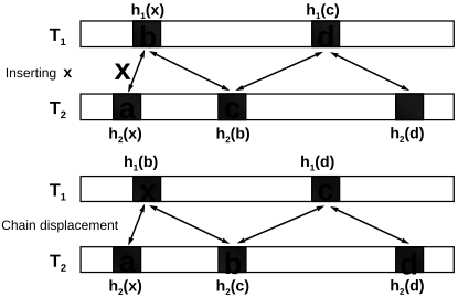
Cuckoo hashing [Pagh and Rodler, 2001] is a technique for resolving collisions in hash tables. The basic idea is to use two irrelevant hash functions to locate two possible buckets in the hash table for each key. When a new key is inserted with its two possible locations being occupied, the collision is resolved by picking either conflicting entry and move it to its alternative location. This procedure may be repeated multiple times (called chain displacement) until a vacant location is found. Figure 1 illustrates an example of collision resolution which causes the chain displacement. As shown, both hashed locations of x are occupied (by a and b) when it is inserted. To resolve the conflict, b is moved to its alternative location, which subsequently causes c and then d being moved to their alternative locations.
Theoretical results show that the amortized operations for resolving each collision is only a small constant, and the failure rate for this procedure (i.e. infinite loop occurs) is in O(1/n) level, which is negligible, when the load factor is less than 50%. By using more than two hashing functions in Cuckoo hashing the load factor can be further improved to more than 90% [Kutzelnigg, 2006]. Recently, Cuckoo hashing has been used as an exact index alternate to feature hashing in sparse feature processing [Zhou et al., 2015], where the feature dimensionality is not reduced. In this paper, we further leveraging Cuckoo hashing for reducing the dimensionality with minimized information loss.
3 Cuckoo Feature Hashing
In this section, we address the technical challenges raised earlier, and introduce the proposed feature hashing method, Cuckoo Feature Hashing (CCFH).
3.1 Feature Hashing viaWeight Sharing
Feature hashing can be interpreted as weight sharing for model parameters [Chen et al., 2015] in machine learning. In practice, the parameter to be learnt is φ(w) ∈ Rk instead of w ∈ Rd . It is equivalent to randomly grouping the features into the hashed dimensions in Rk and having those within the same dimension share the same weight parameter.
Let w ∈ Rd denote the actual feature weights that are applied on the feature set x, and v ∈ Rk denote the parameter to learn in the hashed space. The general goal of weight sharing is to build a mapping F(·) : Rk → Rd to "recover" the parameter w in original space Rd using the hashed representation v. For feature hashing, it is equivalent to the weight sharing scheme w = F(v) where:
Using φ(w) as the parameter v, and using [φ(x)]i to denote the i-th element in φ(x), we have:
There is only a slight difference between feature hashing which computes vT φ(x) and weight sharing which computes F(v)T x, i.e. the dimensionality of x is d and is much larger than the dimensionality of φ(x) which is k. However, considering that both x and φ(x) are sparse representations and have same number of non-zero values, they are just two sides of the same coin. By transforming the problem from feature hashing to weight sharing, we can design operations based on the learnt parameters instead of the original input features.
3.2 Model Design
CCFH uses two hash functions h1(·) and h2(·). Then, the weight of any wi is decided by two reference weights vh1(i)
and vh2(i). In Cuckoo hashing, the key is stored in the hash buckets. Hence, its key-value pair can be directly accessed from the two possible locations in the bucket. In CCFH, to retrieve the actual weight of the parameter wi, we need a binary indicator pi for wi such that
Compared with feature hashing, the parameter retrieved from vh(i) is replaced by a combination of two parameters in the hashed space. When pi is set to 1, the feature weight wi equals to vh1(i); When pi is set to 0, the feature weight wi equals to the parameter vh2(i) in the alternative bucket h2(i).
Obviously, using d indicators for k parameters is excessive. Moreover, discrete parameters are hard to optimize. In CCFH, we propose to hash the indicators and treat them as continuous parameters in the range [0, 1]. Using an additional random hashing function H(·), and considering p ∈ Rd as parameters like w, we apply the weight sharing scheme on it by hashing it to a hashed parameter representation q ∈ [0, 1]l : pi = qH(i), where l should be O(k). The parameter sharing relations for CCFH can then be described as:
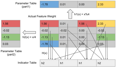
Therefore, the weight sharing relations q are also represented as a set of parameters and can be learnt from the training procedure via gradient based algorithms. Figure 2 shows an example where features in the same column are hashed into the same bucket for h1, and that in the same row are hashed together for h2.
The training of CCFH with parameters v and p is almost equivalent to the training of the original model with parameter w. First, at each time when parameter wi is used (i.e. xi has a non-zero value), it is computed from vh1(i), vh2(i), qH(i) and s(i) using Equation (14). The computation of ∂L ∂w is the same as the gradient computation in the original model. To compute the gradient of the loss L over the parameters v and q, we can utilize the chain rule:
To be specific, we have:
Note that ∂L ∂wi is non-zero only when x is non-zero. Therefore the gradient updates for CCFH only involves constant operations per non-zero input feature.
3.3 Collision Resolving and Sparsity Preserving
Here we discuss how the aforementioned training procedure can mimic the collision resolving operations in Cuckoo hashing. Suppose wa and wb are the two weights of predictive features hashed to the same bucket (e.g., h1(a) = h1(b) = c and qH(a) = qH(b) = 1), and their alternative locations are vh2(a) and vh2(b). At the beginning of training, all parameters including vh2(a) and vh2(b) are starting from near zero value. If these two weights have conflicting optimization interests, ∂L ∂wa and ∂L ∂wb have the opposite sign. Therefore, ∂L ∂qH(a) and ∂L ∂qH(b) also have the opposite sign, suggesting that one of them is negative. The collision between wa and wb is resolved when qH(a) or qH(b) is decreased to 0. If, unfortunately, the collision happens again in vh2(a) or vh2(b), then the above procedure is repeated. Similar scheme works when there are some collisions on the indicator parameters q: suppose qH(a) is moving towards 1 due to collisions of other parameters but wa is expected to be the weight of vh2(a), as long as the weight of vh1(a) is not shared with other predictive features, there will be a derivative on vh1(a) towards the value of vh2(a), and wa will share weight with vh1(a) instead. Although the collision resolving for v and q may contradict each other and lead to a higher failure rate, it is still significantly superior than fixed hashing function where the collision rate equals to the load factor.
Resolving collisions is not the only reason to use CCFH. The performance degradation is not only caused by the collisions between predictive features but also by loss of model sparsity. For example, in multiple hashing, the weightsharing scheme makes more features to share weight with predictive features, henceforth further hurts the model sparsity. Note that the non-zero weight assignment for nonpredictive features should be considered as noises which lead to performance degradation of the model. In CCFH, every feature has two possible weights to choose. Thus, given a load factor of p for predictive features, other features have 1 - p2 chance to be located with near-zero weight (in feature hashing the probability is 1 - p), or be put at the one with smaller absolute value in other cases. Therefore, CCFH not only resolves collisions between predictive features, but also locates most other features at near-zero weight. We have further validated the sparsity analysis above by experimentally evaluating the model sparsity for different methods (see Section 4.4).
| Methods | 1/8M | 1/4M | 1/2M | 1M | 2M | 4M | 81M | 1/8M | 1/4M | 1/2M | 1M | 2M | 4M | 130M |
|---|---|---|---|---|---|---|---|---|---|---|---|---|---|---|
| Exact | - | - | - | - | - | - | 1.46 | - | - | - | - | - | - | .390 |
| FH | 3.15 | 2.64 | 2.21 | 1.97 | 1.75 | 1.64 | - | .429 | .423 | .419 | .411 | .404 | .400 | - |
| MFH2 | 2.78 | 2.35 | 2.08 | 1.87 | 1.67 | 1.60 | - | .425 | .421 | .416 | .409 | .402 | .397 | - |
| MFH4 | 2.84 | 2.34 | 2.06 | 1.84 | 1.63 | 1.58 | - | .428 | .423 | .416 | .408 | .402 | .395 | - |
| CCFH | 2.11 | 1.85 | 1.64 | 1.53 | 1.49 | 1.47 | - | .411 | .405 | .399 | .394 | .392 | .390 | - |
(a) Error Rate(%) on URL
(b) Log Loss on Avazu
Table 1: Main Comparison: Model performance with different model size
4 Experimental Study
4.1 Setup
Dataset. URL [Ma et al., 2009] is a dataset for malicious URL detection. It consists of 2.4 million URLs in total. There are 1.8 million lexical features, 1.2 million host name features and 78 million second order features generated by feature engineering. Each URL contains 300 features on average. Error rate is the conventional evaluation metric. Avazu [Juan et al., 2016] is a dataset for mobile Ads CTR prediction from Kaggle competition. It consists of 40 million samples in total. 130 million features are generated by feature engineering. Each sample contains 550 features on average. Log loss is the evaluation metric suggested by Kaggle.
| Dataset | #Samples | #Features | AvgFeatures | Metric |
|---|---|---|---|---|
| URL | 2.4M | 81M | 300 | Error rate |
| Avazu | 40M | 130M Table 2: | 550 Datasets | Log loss |
Model. We apply logistic regression as the analytics model. Exact index (Exact), feature hashing (FH), multiple feature hashing (MFH) and Cuckoo feature hashing (CCFH) are used to process those sparse feature datasets. Exact index is the exact logistic regression model which explicitly parameterizes every appeared feature. We use dense array and an index dictionary for the implementation. There are some other exact index methods such as [Zhou et al., 2015] which could be more computational efficient. However, their accuracy should be the same. All other methods aim to hash the high-dimension features into a lower dimensional space. We vary their hash-table size (i.e. number of parameters) from 0.125M to 4M and evaluate their accuracy. Two versions of MFH are developed, with 2/4 hashing functions respectively (denoted by MFH2/MFH4). For CCFH, we split the parameter space as two part: 80% for feature weight v and 20% for weight indicator q.
Training Settings. All models are trained using mini-batch stochastic gradient descent (SGD). The batch-size is set to 256, and the learning rate is adjusted based on Adam [Kingma and Ba, 2014] with a momentum of 0.9. L1-penalty is applied to the model parameter as used in [Weinberger et al., 2009; Zhou et al., 2015] to introduce model sparsity (i.e. feature selection).
4.2 Main Results
The test error rate on the URL dataset and log loss on the Avazu dataset are reported in Table ??. MFH solutions do lead to an improvement over FH. However, an FH solution with double parameter size can always outperform the MFH one. This observation can be easily explained as that MFH4 can at most reduce the approximation error by half, while sacrificing the model sparsity. However, doubling the parameter size directly reduces the collision rate by half. Moreover, although MFH2 outperforms FH in all the settings, it is not true between MFH4 and MFH2. MFH4 performs slightly better when the parameter size is large and MFH2 performs slightly better when the parameter size is small. Therefore, resolving the collisions by using more hashing functions is not always cost-effective, due to its limited improvement and significant computation overhead. CCFH achieves the best performance on all the detailed comparisons. With 2/4M parameters, CCFH achieves similar performance compared with the exact index approach which requires a huge feature index and million-scale parameters.
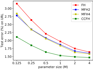
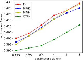
Figure 3 shows the trade-off between model size and model accuracy on URL dataset. To achieve the same level of performance, CCFH only needs at most 1/4 of the model size compared with MFH, and at most 1/8 of the model size compared with FH. Moreover, unlike FH and MFH where the collision rate is inversely proportional to the hash table size, CCFH is expected to resolve most of the collisions between predictive features when the load factor of predictive features is less than a certain threshold. This trend can also be observed from the figure, since the error rate of CCFH rapidly reduces to the floor level when the hash-table size is larger than 1M. All the aforementioned trends can also be observed in Figure 4, which shows the trade-off on Avazu dataset.
4.3 Processing Time
| Data Source | Size | RandomAccess Time |
|---|---|---|
| L1 Cache | 128KB | ∼ 4 cycles |
| L2 Cache | 2MB | ∼ 10 cycles |
| Local L3 Cache | 3MB | ∼ 40 cycles |
| Remote L3 Cache | 30MB | ∼ 70 cycles |
| DRAM | - | ∼ 200 cycles |
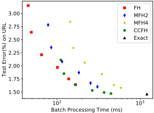
The major advantages of feature hashing include not only reduced model size but also fast processing time, i.e. constant processing time per non-zero input feature. Most of the training time is spent on the random accesses of the parameter table. For FH, only one parameter per input feature needs to be accessed based on its hashing function. For MFH with c hashing functions, c parameters per input feature need to be accessed. CCFH needs to access 2 weight locations and 1 indicator location. While CCFH needs 3 times the processing time compared with FH, its smaller parameter size also increases the cache efficiency. Table 3 shows a typical specification for an Intel Xeon CPU. Considering that each parameter is stored as a 4Byte float variable, a model with 0.5MB parameters can fit in L2 cache, and could be up to 7x faster than a 4MB parameter model which can only fit in the remote L3 cache. Figure 5 shows the trade-off between batch processing time and model accuracy. Comparing with FH, CCFH achieves similar performance accuracy and processing time using a smaller parameter size. Comparing with the exact solution which needs to locate every parameter in an index, CCFH with 2/4M parameters obtains similar accuracy with much lower processing time.
| Methods | 1/8M | 1/4M | 1/2M | 1M | 2M | 4M |
|---|---|---|---|---|---|---|
| FH | 51.5 | 47.7 | 42.1 | 38.4 | 34.7 | 31.5 |
| MFH2 | 55.9 | 49.5 | 46.8 | 41.8 | 37.1 | 33.6 |
| MFH4 | 62.5 | 53.3 | 48.2 | 43.9 | 39.5 | 36.7 |
| CCFH | 47.9 | 39.7 | 32.8 | 29.0 | 28.3 | 27.6 |
| Exact | 26.5 of 300 has a norm larger than 0.02 | |||||
4.4 Sparsity
CCFH is expected to preserve model sparsity. Table 4 summarizes the number of activated features per sample for the URL dataset. A feature is to be activated if its weight has a norm larger than 0.02. L1-penalty is applied to the logistic regression so that only 26.5 of 300 features are activated. Since feature hashing methods introduce weight sharing, potentially resulting in near-zero weights for non-predictive features when there are predictive features in the same bucket. Based on our analysis in Section 3.3, with a load factor of p of non-zero weight in parameter table, p of non-predictive feature cannot be located at zero for FH. CCFH can reduce the rate to p2 . For MFH with c hashing functions, the rate increases to 1 - (1-p)c . Therefore, CCFH has a clear advantage in sparsity preserving when p is small. Experimental results show that CCFH has the best sparsity preserving effect among all methods. With parameter size greater than 1M CCFH significantly outperforms FH, suggesting that the load factor is small. When the parameter size is reduced to 1/8M, p becomes larger and the advantage of CCFH compared with FH becomes less significant. MFH is even worse than FH
since its multiple hashing functions result in more collisions.
4.5 Size of Indicator
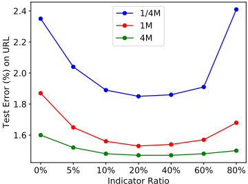
There is only one hyper-parameter for CCFH: the size of indicator q. When no parameter space is split out for q, CCFH degenerates to the MFH2 model. Meanwhile, increasing the size of indicators results in a smaller hash table for feature parameters. We vary the ratio of parameter used as indicators in CCFH with 1/4M, 1M, 4M parameter size. The test error on URL is reported in Figure 6. The performance peaks at 20 - 40%, and is very stable when the ratio is between 10 - 60%.
5 Conclusion
We introduce a novel feature hashing scheme called Cuckoo Feature Hashing(CCFH) to process large scale sparse features. CCFH determines the locations of predictive features during model training, where most collisions lead to performance drop can be avoided. CCFH is realized by providing multiple possible hash locations for each feature, and use indicator parameters to mimic the Cuckoo hashing collision resolving scheme. CCFH is also sparsity preserving and computationally efficient. Experiments on two hundred million features dataset show that CCFH can achieve the similar performance by using only 15%-25% parameters compared with feature hashing.
Acknowledgements
This work is supported by National Research Foundation, Prime Ministers Office, Singapore under CRP Award No. NRF-CRP8-2011-08. Yanyan Shen is supported in part by NSFC (No. 61602297). Wang-Chien Lee is supported in part by the National Science Foundation under Grant No. IIS1717084.
@inproceedings{ijcai2018p295,
  title     = {Cuckoo Feature Hashing: Dynamic Weight Sharing for Sparse Analytics},
  author    = {Gao, Jinyang and Ooi, Beng Chin and Shen, Yanyan and Lee, Wang-Chien},
  booktitle = {Proceedings of the Twenty-Seventh International Joint Conference on
               Artificial Intelligence, {IJCAI-18}},
  publisher = {International Joint Conferences on Artificial Intelligence Organization},
  editor    = {Jérôme Lang},
  pages     = {2135--2141},
  year      = {2018},
  month     = {7},
  note      = {Main track},
  doi       = {10.24963/ijcai.2018/295},
  url       = {https://doi.org/10.24963/ijcai.2018/295},
}
TY - CPAPER TI - Cuckoo Feature Hashing: Dynamic Weight Sharing for Sparse Analytics AU - Gao, Jinyang AU - Ooi, Beng Chin AU - Shen, Yanyan AU - Lee, Wang-Chien T2 - Proceedings of the Twenty-Seventh International Joint Conference on Artificial Intelligence, IJCAI-18 PB - International Joint Conferences on Artificial Intelligence Organization PY - 2018 SP - 2135 EP - 2141 DO - 10.24963/ijcai.2018/295 UR - https://doi.org/10.24963/ijcai.2018/295 ER -Copied
Machine-readable versions of this paper, for tools and AI agents:





