
Complementary Binary Quantization for Joint Multiple Indexing
Proceedings of the Twenty-Seventh International Joint Conference on Artificial Intelligence. Main track. Pages 2114-2120.
https://doi.org/10.24963/ijcai.2018/292
Keywords
- Machine Learning: Unsupervised Learning
- Heuristic Search and Game Playing: Heuristic Search and Machine Learning
- Computer Vision: Recognition: Detection, Categorization, Indexing, Matching, Retrieval, Semantic Interpretation
- Computer Vision: Computer Vision
Abstract
Building multiple hash tables has been proven a successful technique for indexing massive databases, which can guarantee a desired level of overall performance. However, existing hash based multi-indexing methods suffer from the heavy redundancy, without strong table complementarity and effective hash code learning. To address the problems, this paper proposes a complementary binary quantization (CBQ) method to jointly learning multiple hash tables. It exploits the power of incomplete binary coding based on prototypes to align the original space and the Hamming space, and further utilizes the nature of multi-indexing search to jointly reduce the quantization loss based on the prototype based hash function. Our alternating optimization adaptively discovers the complementary prototype sets and the corresponding code sets of a varying size in an efficient way, which together robustly approximate the data relations. Our method can be naturally generalized to the product space for long hash codes. Extensive experiments carried out on two popular large-scale tasks including Euclidean and semantic nearest neighbor search demonstrate that the proposed CBQ method enjoys the strong table complementarity and significantly outperforms the state-of-the-art, with up to 57.76\% performance gains relatively.
- [Cheng et al., 2014] Jian Cheng, Cong Leng, Jiaxiang Wu, Hainan Cui, and Hanqing Lu. Fast and accurate image matching with cascade hashing for 3d reconstruction. In IEEE CVPR, pages 4321-4328, 2014.
- [Datar et al., 2004] Mayur Datar, Nicole Immorlica, Piotr Indyk, and Vahab S. Mirrokni. Locality-sensitive hash- ing scheme based on p-stable distributions. In SCG, pages 253-262, 2004.
- [Gong and Lazebnik, 2011] Yunchao Gong and S. Lazebnik. Iterative quantization: A procrustean approach to learning binary codes. In IEEE CVPR, pages 817-824, 2011.
- [He et al., 2012] Junfeng He, Jinyuan Feng, Xianglong Li- u, Tao Cheng, Tai-Hsu Lin, Hyunjin Chung, and Shih-Fu Chang. Mobile product search with bag of hash bits and boundary reranking. In IEEE CVPR, pages 3005-3012, 2012.
- [He et al., 2013] Kaiming He, Fang Wen, and Jian Sun. K-means hashing: An affinity-preserving quantization method for learning binary compact codes. In IEEE CVPR, pages 2938-2945, 2013.
- [Heo et al., 2012] Jae-Pil Heo, Youngwoon Lee, Junfeng He, Shih-Fu Chang, and Sung-Eui Yoon. Spherical hashing. In IEEE CVPR, pages 2957-2964, 2012.
- [Huang et al., 2013] Long-Kai Huang, Qiang Yang, and Wei-Shi Zheng. Online hashing. In IJCAI, pages 1422- 1428, 2013.
- [Indyk and Motwani, 1998] Piotr Indyk and Rajeev Mot- wani. Approximate nearest neighbors: towards removing the curse of dimensionality. In ACM STOC, pages 604- 613, 1998.
- [Jain et al., 2010] Prateek Jain, Sudheendra Vijaya- narasimhan, and Kristen Grauman. Hashing Hyperplane Queries to Near Points with Applications to Large-Scale Active Learning. In NIPS, pages 928-936. 2010.
- [Jegou et al., 2011] Herve Jegou, Matthijs Douze, and Cordelia Schmid. Product quantization for nearest neigh- bor search. IEEE TPAMI, 33(1):117-128, January 2011.
- [Jiang and Li, 2015] Qing-Yuan Jiang and Wu-Jun Li. Scal- able graph hashing with feature transformation. In IJCAI, pages 2248-2254, 2015. IJCAI
- [Li et al., 2016] Zhujin Li, Xianglong Liu, Junjie Wu, and Hao Su. Adaptive binary quantization for fast nearest neighbor search. In ECAI, pages 64-72, 2016.
- [Lin et al., 2016] K. Lin, J. Lu, C. S. Chen, and J. Zhou. Learning compact binary descriptors with unsupervised deep neural networks. In CVPR, pages 1183-1192, 2016.
- [Liu et al., 2013] Xianglong Liu, Junfeng He, and Bo Lang. Reciprocal Hash Tables for Nearest Neighbor Search. In AAAI, pages 626-632, 2013.
- [Liu et al., 2015] Xianglong Liu, Lei Huang, Cheng Deng, Jiwen Lu, and Bo Lang. Multi-view complementary hash tables for nearest neighbor search. In IEEE ICCV, pages 1107-1115, 2015.
- [Liu et al., 2017] Xianglong Liu, Cheng Deng, Yadong Mu, and Zhujin Li. Boosting complementary hash tables for fast nearest neighbor search. In AAAI, pages 4183-4189, 2017.
- [Mu et al., 2014] Yadong Mu, Gang Hua, Wei Fan, and Shih- Fu Chang. Hash-svm: Scalable kernel machines for large- scale visual classification. In IEEE CVPR, pages 979-986, 2014.
- [Norouzi et al., 2012] Mohammad Norouzi, Ali Punjani, and David J. Fleet. Fast search in hamming space with multi- index hashing. In IEEE CVPR, pages 3108-3115, 2012.
- [Shen et al., 2015] Fumin Shen, Chunhua Shen, Wei Liu, and Heng Tao Shen. Supervised discrete hashing. In IEEE CVPR, pages 37-45, 2015.
- [Song et al., 2013] Jingkuan Song, Yang Yang, Yi Yang, Z- i Huang, and Heng Tao Shen. Inter-media hashing for large-scale retrieval from heterogeneous data sources. In ACM SIGMOD, pages 785-796, 2013.
- [Takebe et al., 2015] Hiroaki Takebe, Yusuke Uehara, and Seiichi Uchida. Efficient anchor graph hashing with data- dependent anchor selection. IEICE Transactions, 98- D(11):2030-2033, 2015.
- [Wang et al., 2015] Qifan Wang, Luo Si, and Bin Shen. Learning to hash on structured data. In AAAI, pages 3066- 3072, 2015.
- [Wang et al., 2018] Jingdong Wang, Ting Zhang, Jingkuan Song, Nicu Sebe, and Heng Tao Shen. A survey on learn- ing to hash. IEEE TPAMI, 40(4):769-790, 2018.
- [Weiss et al., 2008] Yair Weiss, Antonio Torralba, and Rob Fergus. Spectral hashing. In NIPS, pages 1-8, 2008.
- [Xia et al., 2013] Yan Xia, Kaiming He, Fang Wen, and Jian Sun. Joint inverted indexing. In IEEE ICCV, pages 3416- 3423, 2013.
- [Xu et al., 2011] Hao Xu, Jingdong Wang, Zhu Li, Gang Zeng, Shipeng Li, and Nenghai Yu. Complementary hash- ing for approximate nearest neighbor search. In IEEE IC- CV, pages 1631-1638, 2011.
- [Zhang et al., 2014] Ting Zhang, Chao Du, and Jingdong Wang. Composite quantization for approximate nearest neighbor search. In ICML, pages 838-846, 2014.
- [Zhang et al., 2016] Hanwang Zhang, Fumin Shen, Wei Liu, Xiangnan He, Huanbo Luan, and Tat-Seng Chua. Discrete collaborative filtering. In ACM SIGIR, pages 1-10, 2016.
- [Zhu et al., 2016] Han Zhu, Mingsheng Long, Jianmin Wang, and Yue Cao. Deep hashing network for efficient similarity retrieval. In AAAI, pages 2415-2421, 2016.
References were extracted automatically from the PDF and may contain errors.
Full text extracted automatically from the PDF; figures, tables and equations may differ. The PDF is the version of record.
1 Introduction
Nearest neighbor search plays an important role in many areas like large-scale visual search [Xu et al., 2011; Song et al., 2013; Zhang et al., 2014; Wang et al., 2015], machine learning [Jain et al., 2010; Mu et al., 2014], data mining [Zhang et al., 2016], etc. Nowadays, as the amount of data and information explodes, to solve the problem over gigantic database, the hashing[Wang et al., 2018] based approximate nearest neighbors search technique has been widely studied and successfully applied in practice, owing to its compressed storage and efficient computation.
∗Corresponding Author (xlliu@nlsde.buaa.edu.cn)
In the literature, Locality-Sensitive Hashing (LSH) was first introduced in [Indyk and Motwani, 1998; Datar et al., 2004] as one of the most essential concepts. It adopted the random projection paradigm to quantize the data into the binary bit (-1 or 1), promising that the nearest neighbors share the similar codes. The binary codes serve as a type of compact feature descriptor, which helps enable fast search. To further improve the discriminative power of the hash codes, later studies have tried to learn the projections by leveraging the information contained in the data [Weiss et al., 2008; Gong and Lazebnik, 2011; Xu et al., 2011; Huang et al., 2013; Jiang and Li, 2015; Shen et al., 2015] and achieve very encouraging progress. However, they can hardly capture the complex inherent structures underlying the data, relying on the linear hash functions. The nonlinear solutions such as deep learning based [Zhu et al., 2016; Lin et al., 2016] and the prototype based [Li et al., 2016] have shown their great power in a wide spectrum of tasks, where usually complex data relations exist.
The binary codes can achieve compressed storage and efficient computations. But in practice for a balanced search performance at a desired level, usually it is required to build a number of hash tables to index the gigantic database [He et al., 2012; Norouzi et al., 2012; Xia et al., 2013; Cheng et al., 2014]. As the prior work has pointed out that when building multiple tables using the binary codes generated by the most of existing hashing methods [Xu et al., 2011; Liu et al., 2015], we inevitably encounter heavy redundancy among the tables, and subsequently often need a huge number of tables, at the cost of significant precision drops and heavy computation. To address the problem, Xu et al. and Liu et al. first studied complementary hashing methods to leverage the mutual benefits between tables. More recently, a boosting strategy named BCH was proposed to ensemble multiple tables that can maximally cover the nearest neighbors with theoretical convergence guarantee [Liu et al., 2017].
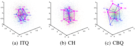
Despite the encouraging progress of complementary multitable indexing, all existing solutions learn the tables in a sequential way, without a overall view of the table relations, and thus still suffer from the table redundancy. Besides, for simplicity they often choose the linear projection based hash functions, which also significantly limit the discriminative power of the hash codes in each table. To address both issues, we develop the prototype based complementary binary quantization (CBQ) that jointly considers the learning of multiple tables. To the best of our knowledge, this is the first work that truly pursues multiple table indices jointly for nearest neighbor search. Figure 1 illustrates the geometric view of the state-of-the-art methods ITQ [Gong and Lazebnik, 2011], CH [Xu et al., 2011], and the proposed CBQ, where CBQ learns evenly distributed binary codes over the whole data space, and thus largely improves the table complementarity by eliminating their redundancy.
2 Complementary Binary Quantization
Next, we will formulate our complementary binary quantization (CBQ) method for joint multi-table indexing.
Before that we first introduce the notations. Suppose we have a training set with n training samples xi ∈ Rd , i = 1 . . . n of d dimension, and let denote the total training data by the matrix X = [x1, x2, . . . , xn] ∈ Rd×n . Our goal is to jointly learn a specific number (i.e., L) of hash functions {h(l) }Ll=1 that can help build informative and complementary hash tables, where each h(l) (·) : Rd ↦→ {-1, 1}b can encode the sample into a b-length binary codes. Namely, the training data X can be encoded as Y(l) = [y(l) 1 , y(l) 2 , . . . , y(l) n ] ∈ {-1, 1}b×n by the l-th hash function.
2.1 Prototype-based Binary Quantization
The prototype technique (e.g., clustering) has been proved very powerful to capture the general metric structure in high dimensional space for large-scale datasets. Therefore, to generate discriminative hash codes for each table, we choose to take advantages of the prototypes to describe the neighbor relations among data. These prototypes will be further assigned unique binary codes for the out-of-sample binary quantization. For multi-table indexing, multiple sets of prototypes will be required which should be able to retrieve the nearest neighbors jointly.
In particular, we learn a set of prototypes P (l) = {p(l) k |p(l) k ∈ Rd } for the l-th table, and each prototype is associated with a unique b-bit binary code c(l) k ∈ {-1, 1}b , forming a binary codebook C (l) ⊆ {-1, 1}b .
Based on the prototypes P (l) and the corresponding codebooks C (l) , any new data point x can be encoded using the code of its nearest prototype in P (l) , according to specific distance function do (usually Euclidean distance). The prototype-based binary quantization function can be defined as follows:
2.2 ComplementaryMulti-Table Quantization
With the prototype-based binary quantization, the problem of learning multiple hash tables can be turn to the pursuit of the prototype sets and their codebooks. We aim to formulate the problem and optimize them jointly.
Multi-Table Quantization Loss
When applying multi-table index to facilitate nearest neighbor search, a true search result can be returned as long as it is retrieved successfully by any hash table. Though directly generating long hash codes using existing hashing methods and then dividing them into multiple parts can also help build multiple tables, our empirical observation shows that usually the data partition generated by different parts tends to be correlated, without considering the nature of the multi-index search.
Motivated by this point, for any sample x we only require at least one of its nearest prototypes in different tables can give the correct search results. Such a nearest prototype can be given by
where do(x, p(l) k ) is the quantization loss of the sample xwith respect to the prototype p(l) k .
As aforementioned, multi-table indexing attempts to maximally utilize the mutual benefits among tables. Therefore, to guarantee the mutual complementarity, we should minimize the following multi-table quantization loss over all the training data
where do(xi, p(l∗ ) k∗ ) ≤ do(xi, p(l) k ), (l, k) ̸= (l∗ , k∗ ).
Based on this formulation, in order to guarantee the strong complementarity, a straightforward way is to reduce the overlaps among the prototypes of different tables.
Space Alignment Loss
Minimizing the multi-table quantization loss can help us find the most discriminative prototypes. However, how to pursue the prototype-based hash functions, that can preserve the original neighbor relations using binary codes, still remains a critical problem.
Both the prototypes and the binary codes can be treated as a kind of data partition, where the prototype works in the original feature space, while the binary code in Hamming space. Therefore, the desired hash functions, encoding the prototypes into binary codes, actually establish a mapping between the original space and the Hamming space. Specifically, we expect the Hamming distances between the binary codes can well approximate the original distances between prototypes, i.e., the following fact should hold:
where dh(c(l′ ) k′ , c(l) k ) is the square root of the Hamming distance between c(l′ ) k′ and c(l) k , and λ is a dynamic scale variable for the two spaces.
Based on this fact, for each sample xi we expect its distance to any prototype p(l) k can be approximated by their corresponding Hamming distance. To characterize such distance consistency, we introduce the space alignment loss in (5), minimizing which will make both the binary codes and the prototypes well fit the true data distribution.
where P (l) is the number of prototypes for the l-th table and M= ∑Ll=1 |P (l) | is the total number of the prototypes.
We should point out that different from the previous prototype based quantization methods like K-means Hashing (KMH) relying on a codebook corresponding to a complete hypercube[He et al., 2013], our method adaptively selects a part of the hypercube to keep the distance consistency, which shows more flexibility for depicting inherent data structure.
The Formulation
Based on the multi-table quantization loss and the space alignment loss, we can obtain our final formulation for complementary binary quantization:
Here, the first constraint on the binary codes in each C (l) will guarantee that each prototype will be assigned a unique code. Besides, for each sample xi, the second constraint allows us mainly focus on the capability of its nearest prototype, which is suitable for the multi-indexing search.
3 Joint Table Learning
There are multiple sets of prototypes and codebooks evolved in Problem (6), which are coupled due to the multi-indexing constraints. Moreover, the pursuit of the discrete binary codes further increase the complexity of the problem. Therefore, usually it is quite hard to directly solve it. Fortunately, by transforming the multi-table quantization to a joint one, we can address the above issues using an efficient alternating optimization algorithm and jointly learn multiple tables for a small b (e.g., b ≤ 4).
3.1 ProblemReformulation
Since our goal is to jointly optimize all prototypes and codebooks of multiple hash tables, we first attempt to reformulate the pursuit of multiple prototype sets to the learning of one joined prototype set.
Since in multi-table search we only focus on the nearest prototype across all tables for each query sample as formulated in Problem (6), this can be done by merging all prototype sets P (l) into a larger one P = ∪P (l) and then finding the nearest prototype from it. Correspondingly, their codebook sets can also be joined as one C = ∪C (l) with repetition. Note that, in C there will be the possibility that the same binary code occurs multiple times, and the total occurrence times for each unique code should be less than L.
Based on this fact, we can construct a one-to-one mapping that converts the original prototype index (l, k) to a uniform one m ∈ {1, 2, . . . ,M}. Subsequently, both the multi-table quantization loss and the space alignment loss can be rewritten as follows:
where π(cm) denotes occurrence time for the code cm. m∗i is uniform index of prototype which is closest to sample xi.
3.2 Alternating Optimization
With the new formulation, now we can present an efficient alternating optimization algorithm.
Step 1: Incomplete Coding
First, suppose we already have the prototypes and the assignment for each sample (to start the algorithm, we initialize them as described in Section 3.3). The problem turns to encoding the prototypes using a subset of binary codes from L hypercubes (with L× 2b candidate codes) that can align the spaces. Such an incomplete coding idea prove to be able to fit the true data distribution using a part of hypercube structure for each table.
Specifically, if supposing in the prototype set P, a subset of prototypes p1, ...pm have been assigned the binary codes c1, ...cm(1 ≤ m ≤ M), then we attempt to find the optimal binary code cm′ for prototype pm′ from the remaining binary codes Cr = ⋃L{-1, 1}b - {c1, . . . , cm}. With the fact that 1n ∑ni=1 d2o (xi, pm∗i ) is a constant, the problem in (7) is equivalent to:
Since there are at most 2b candidate codes for each prototype, the incomplete coding can be directly solved by evaluating the loss for each candidate and selecting the minimal one by a greedy algorithm. For m = 1 as the start of the coding, we can choose any binary code c1 for any prototype, owing to the high symmetry of the hypercube structure.
Step 2: Prototype Pursuit
After obtaining the codebook C, next we can update the prototype set P to further reduce the multi-table quantization loss and increase the space consistency. Therefore, we have the following subproblem:
The above problem is quite similar to the classic k-means clustering. Motivated by this observation, we can simply optimize the subproblem by iteratively updating the prototype and the assignment for each sample. Specifically, by fixing the assignment we can derive the update of pm as follows:
where wm is the number of samples assigned to the prototype pm. The optimal assignment for each sample xi in multitable search can be found easily as we pointed before:
Note that the prototype set will shrink, due to that some uninformative prototypes without any sample assigned will be abandoned. This will lead to the incomplete coding.
Step 3: Rescaling
The learnt prototype and codebook sets respectively construct a distribution structure in original data space and Hamming space. Intuitively, by minimizing the space alignment loss, the two structures can be well matched. To further minimizing the quantization loss, we still require a proper space scaling that make the distance measurement consistent across the two spaces. This can be completed by solving the following subproblem.
whose optimal solution can be given by
Table Assignment
After we jointly optimize the prototypes P and hash codebook C, to build L hash table indices we can simply divide them to L parts using a random assignment strategy, following the two principles: (1) there are no identical hash codes in
Algorithm 1 Complementary Binary Quantization (CBQ).
Input: Training set X, hash table number L, code length b per table.
Output: Hash functions {h(l) }Ll=1
- 1: Initialize prototype set P and the assignment index m∗i for X using K-means.
- 2: Initialize the scale variable λ according to (14).
- 3: repeat
- 4: for m′ = 1, 2, . . . ,M do
- 5: Update the code set C using the local optimal binary code cm′ for pm′ by solving (8).
- 6: end for
- 7: Update P by iteratively solving (10) and (11).
- 8: Update λ according to (13).
- 9: until convergence
- 10: Assign P and C to L hash tables, generating {h(l) }Ll=1 .
the same hash table, and (2) the prototype numbers of every hash table should be balanced.
Since each binary code corresponds to an integer number varying in {0, 1, . . . , 2b - 1}, we conduct the assignment according to their numerical order. Namely, we allocate the hash codes and the prototypes with the same number to different tables, which promises that the same hash codes will not appear in the same table. Besides, we try to keep the number of the assigned codes in each table evenly distributed, and thus balance the indexing capability of multiple tables.
Algorithm 1 lists the main optimization steps of our CBQ method for the joint multi-table learning.
3.3 Discussions
Initialization
To start the algorithm, we initialize the prototypes P and the assignment m∗i for each samples using the classical K-means algorithm on the training data set. The number of clusters (or prototypes) is set to M = L × 2b at first. Based on the initialization, we also estimate the scaling variable λ using the full binary codes in L hypercubes of b dimension, i.e., similar to (13),
Generating Long Hash Codes
Till now we have discuss how to generate multiple complementary hash tables, each of which relies on a short hash codes (usually b ≤ 4). In practice, often long binary codes are required in many tasks for a better performance. However, it is difficult for our CBQ to jointly learns L× 2b′ prototypes for a large b′ > 4, due to the exponential computation. Fortunately, in our paper we mainly focus on the generic Euclidean distance and thus can adopt the popular product quantization (PQ) technique to generalize CBQ to product space for long binary codes. Specifically, in order to generate long hash codes, we can first divide the original space into multiple subspaces, then learn a small codes using our CBQ method, and finally concatenate the small ones in different subspaces to the long ones in a Cartesian product manner.
| METHOD | SIFT-1M | GIST-1M | ||||||||
|---|---|---|---|---|---|---|---|---|---|---|
| L=1 | L=4 | L=8 | L=16 | TRAIN TIME | L=1 | L=4 | L=8 | L=16 | TRAIN TIME | |
| LSH | 27.71 ±0.63 | 29.40 ±0.81 | 29.08 ±2.47 | 29.62 ±0.79 | 0.04 | 9.67 ±0.61 | 10.54 ±0.42 | 11.54 ±0.24 | 11.76 ±0.84 | 5.11 |
| ITQ | 41.06 ±1.53 | 30.70 ±0.33 | - | - | 3.40 | 26.83 ±0.28 | 16.62 ±0.60 | 14.20 ±0.31 | 12.59 ±0.80 | 12.83 |
| SH | 48.81 ±0.84 | 19.64 ±3.32 | 14.55 ±2.59 | 10.53 ±0.87 | 0.19 | 13.72 ±1.10 | 8.05 ±1.13 | 5.90 ±0.57 | 4.97 ±0.44 | 2.22 |
| AGH | 31.55 ±1.71 | 30.01 ±1.91 | 28.07 ±1.79 | - | 0.40 | 12.55 ±1.25 | 11.28 ±0.50 | 11.62 ±0.50 | - | 4.51 |
| SPH | 39.41 ±0.89 | 41.49 ±0.59 | 41.78 ±0.98 | 41.61 ±0.38 | 5.30 | 22.76 ±0.59 | 19.68 ±0.52 | 19.50 ±0.44 | 19.42 ±0.55 | 18.39 |
| ABQ | 51.53 ±1.30 | 32.88 ±0.57 | 24.61 ±0.69 | 10.60 ±0.61 | 36.08 | 29.28 ±0.60 | 17.44 ±0.55 | 14.22 ±0.67 | 4.56 ±0.06 | 74.00 |
| CH | 50.51 ±0.94 | 52.28 ±0.35 | 53.05 ±0.80 | 54.12 ±0.82 | 0.24 | 18.74 ±0.78 | 23.83 ±0.41 | 24.74 ±0.41 | 25.68 ±0.53 | 2.94 |
| BCH | 45.81 ±0.93 | 53.30 ±0.44 | 55.69 ±0.60 | 57.37 ±0.31 | 258.33 | 14.02 ±0.65 | 17.04 ±0.40 | 18.59 ±0.60 | 19.94 ±0.71 | 332.61 |
| CBQ(OURS) | 52.39 ±0.71 | 55.95 ±0.68 | 57.38 ±0.51 | 57.76 ±0.79 | 18.75 | 26.55 ±1.09 | 28.87 ±0.72 | 29.28 ±1.18 | 29.38 ±0.83 | 27.51 |
Complexity
To learn L hash tables from n training samples of d dimension, our CBQ algorithm will totally spend O(4bndL2 ) time on the incomplete coding (step 1) that greedily finds the locally optimal code for each prototype in each subspace, and at most 4bndL2 time on prototype (step 2) and scalar update (step 3), mainly deriving from the computation of the distances between training samples and prototypes. With the short code length b ≤ 4 of each subspace, the term 4bL2 can be treated as a constant. Therefore, the total time for training is linear to the size of the training set. At the online search stage, for each query point the hash functions need O(2bdL) time to compute the nearest prototype and O(1) time for the code assignment. This is almost the same to the fast hashing methods like LSH and ITQ.
4 Experiments
In this section we will evaluate the proposed Complementary Binary Quantization (CBQ) in two popular large-scale tasks including Euclidean and semantic nearest neighbor search.
We first compare CBQ to the state-of-the-art well-known unsupervised hashing algorithms, including the projection based ones like Local Sensitive Hashing (LSH)[Indyk and Motwani, 1998], Iterative Quantization (ITQ)[Gong and Lazebnik, 2011], Spectral Hashing (SH)[Weiss et al., 2008] and Anchor Graph Hashing (AGH)[Takebe et al., 2015], and two representative prototype based ones including Spherical Hashing (SPH)[Heo et al., 2012] and Adaptive Binary Quantization (ABQ)[Li et al., 2016]. Besides, since we mainly tackle the multiple table indexing problem from the practical view, which is quite different from the conventional hashing methods, we also compare our CBQ with two state-of-theart multi-table methods including Complementary Hashing (CH)[Xu et al., 2011] and Boosting Complementary Hashing (BCH)[Liu et al., 2017].
We have to point out that most of the existing hashing research mainly devoted their efforts to pursuing compact hash codes for Hamming distance ranking or single hash table lookup. Therefore, when applying these methods to building L (L = 1, 4, 8, 16) tables with b-length (b = 24) hash codes in each table, we adopt the common strategy that first generates bL-length codes totally and then equally divides them to L parts correspondingly forming L hash tables, similar to Multi-Index Hashing [Norouzi et al., 2012]. For those methods using PQ subspace (ABQ and CBQ), we encode the data in each subspace using 3 bits.
4.1 Evaluation Protocols
In the following experiments we respectively build a different number of hash tables using different methods. As we mainly focus on multi-table indexing technique, we adopt two search schemes over the multiple hash tables, namely the Hamming distance ranking and the hash table lookup.
The Hamming distance ranking should reflect the nature of multi-table search that a point in any hash table with a small Hamming distance to the query will be ranked top. Formally, for the query xq and any database point xi we can give their distance over multiple tables as follows
Based on such Hamming distance we can rank all database points in the multi-table indexing nature, and evaluate the ranking performance in terms of the average precision.
Hash table lookup works like the inverted indexing, where the points falling within a small Hamming radius r (usually r ≤ 2 for efficiency) from the query code are retrieved from each table and merged as the final results. We mainly concern the overall performance by reporting F1-measure.
In the experiments, we randomly select 10,000 and 1,000 samples as the training and the testing set respectively. Besides, to suppress the randomness we repeat all experiments 10 times and report the averaged performance.
4.2 Results and Discussions
Multi-table indexing serves as a very fundamental technique in the fields of computer vision, information retrieval, etc. Here, we investigate two of its popular applications including feature matching (Euclidean nearest neighbor search) and image retrieval (semantic nearest neighbor search).
Euclidean Nearest Neighbor Search
Here we employ the two widely-used datasets SIFT-1M and GIST-1M [Jegou et al., 2011] that respectively consist of one million 128-D SIFT and 960-D GIST-1M features. In this task, the groundtruth is defined according to Euclidean distance, namely for each query the top 5‰points with the smallest Euclidean distances are regarded as its nearest neighbors. We set µ to 100 on SIFT-1M and 0.2 on GIST-1M.
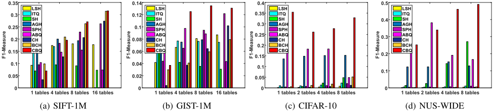
Table 1 lists the average precision of the top 100 with respect to different number of hash tables. From the table, it is easy to see that the multi-table methods significantly outperform conventional hashing methods like ITQ and ABQ when constructing more hash tables. This further validates our conclusion that most of existing hashing methods, mainly focusing on compact binary codes, are not suitable for the multi-indexing task. Note that LSH also improves the performance slightly, and this is why many practical applications build table indexing using LSH instead of the learning based ones. Compared to LSH and the other state-of-the-art multitable methods, our CBQ can obtain the best performance in all cases based on the joint quantization, which indicates that the joint quantization can faithfully help strengthen the complementary between tables. We can get the similar conclusion from Figure 2 (a) and (b), which depict the F1-measure on the two datasets. In Table 1, we also report the training time and find that CBQ enjoys fast training as we analyzed.
| METHOD | CIFAR-10 | NUS-WIDE | ||||||||
|---|---|---|---|---|---|---|---|---|---|---|
| L=1 | L=2 | L=4 | L=8 | TRAIN TIME | L=1 | L=2 | L=4 | L=8 | TRAIN TIME | |
| LSH | 17.58 ±0.76 | 18.40 ±1.10 | 19.85 ±0.65 | 20.74 ±0.70 | 1.17 | 37.96 ±0.50 | 40.61 ±1.76 | 41.34 ±1.64 | 42.22 ±1.22 | 1.13 |
| ITQ | 31.01 ±0.63 | 27.37 ±0.84 | 26.36 ±0.60 | 26.62 ±0.32 | 11.65 | 49.19 ±0.30 | 47.38 ±0.59 | 45.84 ±0.73 | 46.37 ±0.84 | 8.17 |
| SH | 18.22 ±0.87 | 14.84 ±0.91 | 13.03 ±0.18 | 12.65 ±0.25 | 6.86 | 38.43 ±1.32 | 37.41 ±0.69 | 35.22 ±0.68 | 36.39 ±0.57 | 6.32 |
| AGH | 32.23 ±1.39 | 31.11 ±2.51 | 29.14 ±2.42 | 29.44 ±1.24 | 1.93 | 49.62 ±2.66 | 49.22 ±1.80 | 49.70 ±1.00 | 48.53 ±1.79 | 1.69 |
| SPH | 22.64 ±1.38 | 22.17 ±0.29 | 22.03 ±0.44 | 22.55 ±0.13 | 33.95 | 43.21 ±1.22 | 43.71 ±1.07 | 43.67 ±0.66 | 44.08 ±0.82 | 30.13 |
| ABQ | 18.94 ±5.26 | 10.62 ±0.88 | 10.77 ±0.67 | 10.97 ±0.46 | 32.67 | 38.73 ±3.75 | 36.98 ±2.92 | 36.44 ±1.81 | 34.41 ±1.52 | 36.42 |
| CH | 18.48 ±0.27 | 22.02 ±0.82 | 24.75 ±1.34 | 26.11 ±0.36 | 8.12 | 38.46 ±0.59 | 42.32 ±0.56 | 44.52 ±0.71 | 45.72 ±0.83 | 6.90 |
| BCH | 18.52 ±1.10 | 19.95 ±1.06 | 19.22 ±1.69 | 22.44 ±1.18 | 747.89 | 37.95 ±2.54 | 39.46 ±0.86 | 38.70 ±1.48 | 39.07 ±1.96 | 903.97 |
| CBQ(OURS) | 39.66 ±1.79 | 39.37 ±1.89 | 36.63 ±1.51 | 36.62 ±1.22 | 59.60 | 51.92 ±1.53 | 54.08 ±1.86 | 52.18 ±0.91 | 51.14 ±1.76 | 53.69 |
| SIFT-1M | GIST-1M | ||||
|---|---|---|---|---|---|
| METHOD | F1 MEASURE | TIME COST | F1 MEASURE | TIME COST | |
| PQ | 23.18 | 1.22 | 13.12 | 3.39 | |
| CBQ | L=8 | 19.52 | 0.02 | 13.45 | 0.14 |
| L=16 | 27.08 | 0.04 | 13.07 | 0.26 | |
Semantic Nearest Neighbor Search
We further evaluate CBQ on semantic nearest neighbor search for the image retrieval task. we choose two widelyused large-scale image datasets: CIFAR-10 and NUS-WIDE. CIFAR-10 contains of 60K 32×32 color images of 10 classes and 6K images in each class, and NUS-WIDE consists of over 269K images with 81 semantic tags. Here, the groundtruth for each query is defined as those samples with common semantics (class or tag) as the query. For both datasets, we extract 4096-D convolutional features for each image using the pretrained VGG network. For NUS-WIDE, we further select 21 most frequent tags for the task in the NUS-WIDE dataset. We set µ to 10 on CIFAR-10 and 20 on NUS-WIDE.
Table 2 reports the MAP performance using different methods on CIFAR-10 and NUS-WIDE, where we can get the same observation that the multi-table learning methods increase the performance obviously when constructing more hash tables, and while the conventional compact hashing methods usually decrease. Figure 2 (c) and (d) further investigate the F1-measure performance using hash table lookup. In all cases, we can find that our CBQ performs consistently with the best performance among all methods, which proves that our joint quantization solution promises the complementarity for the semantic neighbor relations.
In Table 3, we also compared our CBQ with the inverted indexing based on product quantization. From the table, we can see that when using the same lookup radius, our CBQ using 8 or 16 tables can get the comparable or even better performance. But in practice, CBQ search is much faster than PQ indexing method.
5 Conclusion
In this paper we mainly studied the hash based multi-indexing problem that has been widely used in many large-scale applications, and proposed a complementary binary quantization (CBQ) method that can jointly pursues multiple complementary and informative hash tables. CBQ method simultaneously considers the nature of multi-table search and the alignment between the original and Hamming space, and can preserve the space consistency using multiple tables. Compared to the state-of-the-art multi-table learning methods, it enjoys both fast training and effective coding based on prototypes and the PQ technique. We have comprehensively evaluated our CBQ method on two fundamental tasks including Euclidean and semantic nearest neighbor search, and our results prove that CBQ can significantly outperform the state-of-thearts with strong table complementarity.
Acknowledgments
This work was supported by the National Natural Science Foundation of China (61690202) and MSRA Collaborative Research Grant.
@inproceedings{ijcai2018p292,
  title     = {Complementary Binary Quantization for Joint Multiple Indexing},
  author    = {Fu, Qiang and Han, Xu and Liu, Xianglong and Song, Jingkuan and Deng, Cheng},
  booktitle = {Proceedings of the Twenty-Seventh International Joint Conference on
               Artificial Intelligence, {IJCAI-18}},
  publisher = {International Joint Conferences on Artificial Intelligence Organization},
  editor    = {Jérôme Lang},
  pages     = {2114--2120},
  year      = {2018},
  month     = {7},
  note      = {Main track},
  doi       = {10.24963/ijcai.2018/292},
  url       = {https://doi.org/10.24963/ijcai.2018/292},
}
TY - CPAPER TI - Complementary Binary Quantization for Joint Multiple Indexing AU - Fu, Qiang AU - Han, Xu AU - Liu, Xianglong AU - Song, Jingkuan AU - Deng, Cheng T2 - Proceedings of the Twenty-Seventh International Joint Conference on Artificial Intelligence, IJCAI-18 PB - International Joint Conferences on Artificial Intelligence Organization PY - 2018 SP - 2114 EP - 2120 DO - 10.24963/ijcai.2018/292 UR - https://doi.org/10.24963/ijcai.2018/292 ER -Copied
Machine-readable versions of this paper, for tools and AI agents:





