An Efficient Algorithm To Compute Distance Between Lexicographic Preference Trees

1 Introduction

There are many situations where we have to represent and reason about different agents' preferences over a set of possibly interrelated attributes or variables [Lang et al., 2012; Horniaˇcek, 2008]. For example, one may need to group customers based on their preferences to discover common decision patterns, and recommend actions [Br¨auning et al., 2017]. Several work has been published on clustering and predicting preference/ranking data where the ranking over the training labels (correspond to alternative outcomes) is assumed to be given [H¨ullermeier et al., 2008; Vembu and G¨artner, 2011; Grbovic et al., 2013; Todorovski et al., 2002]. The task then involves the prediction of strict label order relations. This is, however, impractical when a combinatorial domain is involved: i) data collection becomes infeasible when there is a large number of decision attributes. For instance, even with 5 binary attributes, there will be 25 = 32 unique outcomes. If we collect the preference data via pairwise comparison query, there will be (32 2 ) = 496 pairs of outcomes that each user needs to compare. ii) predicting ranking is considered as a complex learning task, as the predicted output is a ranking relation rather than single values like those in traditional ML tasks. More generally, with a combinatorial domain, the number of alternatives grows exponentially fast with the number of attributes. In such case, the output of the algorithm is a huge ranking list over the alternative space. Moreover, in tasks like clustering, it is more meaningful to build explanatory models so that one can examine the intra-cluster attribute preferences and attribute importance structures to discover common decision patterns among agents.

In this paper, we consider lexicographic preference trees (LP-trees) [Wilson, 2006; Booth et al., 2011] for representing agents' preferences over combinatorial domains. LP-trees are one of the most intuitive and compact representations that correspond to many real-world preferences exhibited by human decision makers [Schmitt and Martignon, 2006; Yaman et al., 2008; Wilson, 2014; Liu and Truszczynski, 2015]. They have a variety of potential applications in the current ML era. For example, they can be used as inputs to cluster agents based on agents' preferences, or to predict the satisfaction level of an agent based on similar agents' LPtrees. However, in common ML practices like clustering or prediction, many existing algorithms rely on the assumption that there is a numerical space they can model. For instance, the famous KNN classification [Cover and Hart, 1967] and KMeans clustering algorithms [Hartigan and Wong, 1979] cannot directly classify or cluster LP-trees. They need to measure the distance between any pair of samples while LP-trees do not provide such information per se. Therefore, some transformations are required to extract distance information between LP-trees. Otherwise, many existing ML algorithms are inapplicable.

In this paper, we tackle the problem of calculating the number of pairwise disagreements (commonly called Kendall tau ranking distance) between agents' preferences represented by LP-trees. We propose a novel algorithm, LpDis, to compute the distance between two agents' LP-trees without the need of explicitly generating all possible pairs. It avoids any unnecessary comparisons while preserving the accuracy. Moreover, LpDis is very flexible: it neither poses any restriction on the structures of LP-trees, nor requires agents to share common preference dependencies or importance structures. Experimental results show that LpDis performs very fast and scales well compared to an exhaustive querying method.

In the next section, we provide the preliminaries of LPtrees. We then present the theoretical basis and our algorithm in Section 3 and 4, respectively. At last, we discuss the experimental results in Section 5 and close with conclusions and a brief account of future work in Section 6.

2 Lexicographic Preference And LP-trees

Let V = {X1, · · · ,XN} be a set of N attributes and DX be the domain of an attribute X. When X is binary, we write DX = {x, ¯x}. Let O be the outcome space, i.e., the Cartesian product of attribute domains ∏ X∈V DX. We denote outcomes

as lowercase Greek letters (α, β, etc.). An outcome α ∈ O is represented as a vector α = (x1, · · · , xN) where xi ∈ DXi .

For any subset of attributes X ⊆ V, we write DX = ∏ X∈X DX. We denote the projection of an outcome α on X

as α [X]. For convenience, if X = {X} is a single attribute, we write α [X] instead of α [{X}].

Definition 1 (Consistent assignments). Let x and y be the value assignments to two attribute subsets X and Y, respectively. We call, x is consistent with y, written as x ▷◁ y, if they assign the same values to all common attributes X∩Y (i.e., x[X∩Y] = y[X∩Y]); Otherwise, they are conflicting x ̸▷◁ y, i.e., ∃X ∈ X∩Y such that x[X] ̸= y[X].

Obviously, if Y ∩ X = ∅, we have x ▷◁ y. Also, when Y ⊆ X and x ▷◁ y, we have x[Y] = y.

A lexicographic order on O is a total order induced by two major elements: i) the attribute importance order on V; ii) local preferences on attribute values. It orders a pair of outcomes {α, β} by looking at the attributes in sequence according to their importance, until we reach an attribute X such that the values of X are different between α and β. α and β are then ordered according to the local preference relation over the values of X. This corresponds to the conditional preference theory discussed in [Wilson, 2004], given the assignment u to the more important attributes in both α and β, α ≻ β if and only if α[X] ≻u β[X], irrespective of values assigned to the less important attributes in α and β. In general, both the importance relations between attributes and the attribute preferences can be conditioned on the values of more important attributes. Such lexicographic preference relations can be compactly represented by lexicographic preference trees (LP-trees).

2.1 Lexicographic Preference Trees

According to [Booth et al., 2011], an LP-tree T is a tree where each node n is labelled with an attribute denoted by Vn. Every non-leaf node has between one to a maximum of |DVn | outgoing branches, each with a branching constraint Vn = x (x ∈ DVn ). Every attribute appears exactly once on every branch of the tree. The tree structure defines the importance

̄

̄

̄

̄

relations over attributes: each branch of the tree specifics a descending order (from root to leaf) over attributes. We use ▷ to denote the importance relation over attributes to distinguish it from the preference relation ≻.

There is a conditional preference table (CPT) associated with each node n in an LP-tree, which is defined as follows. Let P be the set of parent attributes where the preferences over the values of Vn would condition on. The CPT of n is then composed of the local preferences over DVn for all valuations of P: {p : x1 ≻ · · · ≻ xk |xi ∈ DVn and p ∈ DP}. p is called a parent context.

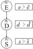
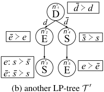
Example 1 (LP-trees). Figure 1 illustrates two different LPtrees T and T ′ for a simple conference flight reservation scenario. We label every node as ni and n′i in T and T ′ respectively. Consider the following binary-valued attributes:

• E - Early departure. e denotes an early trip (e.g., departing at least 2 days earlier); and ¯ e is a just-on-time trip;
• D - Day-time flight. d (resp. ¯ d) denotes a day-time (resp. a night-time) flight;
• S - Stop-over. s (resp. ¯ s) means a stop-over (resp. non-stop) flight.

Figure 1a is a simple LP-tree T where the user considers the departure date (E) as the most important attribute: he prefers an early trip (e ≻ ¯ e); followed by the time of flight (D): he likes a day-time flight more than a night-time flight (d ≻ ¯ d); and at last the stop-over feature (S): he prefers to have some stop-overs (s ≻ ¯ s). Note that in T , the attribute importance and attribute preferences are unconditional.

Figure 1b shows a more general example of LP-tree T ′ , where the user has both conditional attribute importance and conditional attribute preferences. D is the most important attribute, and the user prefers night-time flight over day-time flight ( ¯ d ≻ d). Then, conditioned on the value of D:

• If D = d, the next most important attribute is E (on n′2 ) and ¯ e ≻ e. Then the least important variable is S (on n′3 ), where the CPT of S states that s ≻ ¯ s if E = e; otherwise if E = ¯ e, then ¯ s ≻ s.
• If D = ¯ d, the second most important attribute is S (on n′4 ), and followed by E (on n′5 ). For S (resp. E), the CPT states that ¯ s ≻ s (resp. e ≻ ¯ e).

An LP-tree T induces a total order ≻T on the outcome space O. For a pair of outcomes {α, β}, we query T in a topdown manner, following the relevant branch according to the common value assignment in α and β. Until we reach a node n in T , where α and β have different values assigned to Vn (α[Vn] ̸= β[Vn]). We look into the CPT of n and conclude that α ≻T β if and only if α[Vn] ≻p β[Vn] where p is the parent context of Vn specified in α and β (p = α[P] = β[P]).

Example 2 (Outcome Comparison). Consider the outcome pairs α = ¯ ed¯ s, β = eds, and T ′ in Figure 1b, we query T ′ accordingly. The first visited node is n′1 and Vn′1 = D. As α[D] = β[D] = d, we continue to move to the left child n′2 , where Vn′2 = E. Now, as α[E] ̸= β[E] (α[E] = ¯ e but β[E] = e). According to the CPT on n′2 , we have ¯ e ≻ e. Therefore, we can directly conclude that α ≻T ′ β.

3 Kendall Tau Distance Between LP-trees

A typical ML scenario is to cluster agents based on their preferences, where we need to look into the similarity or distance between different agents' preferences. In this section, we introduce our novel LpDis algorithm that efficiently traverses LP-trees and calculates the number of disagreed pairwise preference relations (Kendall tau ranking distance) between two LP-trees. LpDis has the following advantages:

• (i) It does not restrict the structures of the LP-trees. The LP-trees can have different preference dependencies between attributes and attribute importance structures;
• (ii) It considers general multi-valued domains, instead of restricting to binary-valued attributes;
• (iii) It only traverses the nodes in two LP-trees without the need of generating the entire outcome space or querying LP-trees for any outcome pair. Hence, it significantly improves the computation time, which is crucial in large-scale ML tasks.

3.1 Preference Encoded In LP-tree Nodes

As mentioned earlier, an LP-tree T induces a total order over the outcome space O. This means, for any possible outcome pair {α, β}, it can only be either α ≻T β or β ≻T α. Such pairwise preferences are encoded in the nodes of an LP-tree.

Given an LP-tree T and a node n in T , let A be the set of ancestor attributes of n, B be the set of branching attributes (attributes on nodes that have multiple outgoing edges) along the path to n (B ⊆ A), and b be branching constraints, i.e., the value assigned to B along the path to n. Then, n decides the preference order over a pair of outcomes {α, β} in T if it is the first node where α and β have different values. We denote the set of all such outcome pairs as Pn. For any of these outcome pairs {α, β} ∈ Pn, α and β have the same assignment to A (and with α[B] = β[B] = b), but differ on Vn (i.e., attribute on n), and irrespective of the values assigned to the rest of the descendants of n. Formally,

Note that {α, β} and {β, α} are considered as the same outcome pairs. For any pair of nodes ni, nj in an LP-tree, Pni ∩Pnj = ∅ (i.e., they are disjoint) because every outcome pair {α, β} is decided at exactly one node in the tree: α ≻T β if and only if the CPT of Vn states that α[Vn] ≻p β[Vn] in the parent context p included in α[A] (=β[A]). Also, the sum of |Pn| of all the nodes in an LP-tree, i.e., ∏ n∈T |Pn|, is then

equal to the total number of outcome pairs.

Example 3 (Node Outcome Pairs). Consider node n2 of the LP-tree T in Figure 1a, where Vn2 = D. we have A = {E}, B = ∅. So Pn2 = {{α, β} | α[E] = β[E] and α[D] ̸= β[D]}. Therefore, Pn2 contains the following outcome pairs: {eds, e ¯ ds}, {¯ eds, ¯ e ¯ ds}, {eds, e ¯ d¯ s}, {¯ eds, ¯ e ¯ d¯ s}, {ed¯ s, e ¯ ds}, {¯ ed¯ s, ¯ e ¯ ds}, {ed¯ s, e ¯ d¯ s}, {¯ ed¯ s, ¯ e ¯ d¯ s}. Similarly, consider node n′2 in T ′ in Figure 1b. We have Vn′2 = E, A = B = {D} and b = d. So Pn′2 = {{α, β} | α[D] = β[D] = d and α[E] ̸= β[E]} = {{¯ eds, eds}, {¯ eds, ed¯ s}, {¯ ed¯ s, eds}, {¯ ed¯ s, ed¯ s}}.

3.2 Node Disagreement Between LP-trees

Since two LP-trees could have different attribute importance structures, for any pair of nodes n, n′ in two LP-trees T and T ′ , respectively, Pn and Pn′ could contain different sets of outcome pairs. In the following, we define the set of disagreed outcome pairs between nodes in two LP-trees.

Definition 2 (Disagreed outcome pairs between nodes). Let T , T ′ be two LP-trees, n and n′ be a node in T and T ′ , respectively. The set of disagreed outcome pairs Dn,n′ (equivalent to Dn′ ,n) is defined as follows:

Similar to LP-tree that encodes its preferences using two components (attribute preferences and attribute importance), the disagreement between two LP-trees also occurs because of two reasons: different local preferences on attribute values and different structures of attribute importance.

Given two nodes n and n′ of the LP-trees T and T ′ , respectively, let A (resp. A′ ) be the set of ancestor attributes of n (resp. n′ ), and ˘A be the union of ancestor attributes ˘A = A ∪ A′ . Let B (resp. B′ ) be the set of branching attributes of n (resp. n′ ), and b (resp. b′ ) be the branching constraints of n (resp. n′ ). It is important to note that if b and b′ are conflicting (b ̸▷◁ b′ ), Pn ∩ Pn′ = ∅, i.e., there exists no possible assignment to the joint ancestor ˘A s.t. both b and b′ are True. In this case, |Dn,n′ | = 0. Therefore, when computing the disagreement between pairs of nodes in two LP-trees, we can focus on those where b ▷◁ b′ . Let ˘B be the union ˘B = B ∪ B′ and ˘b be the union of branch constraints specified by n and n′ (assuming b ▷◁ b′ ), then the common outcome pairs in Pn and Pn′ would be those that assign the same values to ˘A, satisfy the joint constraint ˘b but assigns different values to Vn and Vn′ :

Node Disagreement Caused By Local Preference

If n and n′ are both labeled with the same attribute (Vn = Vn′ ), the disagreement between n and n′ is caused by the conflicting local preferences over attribute values DVn . Let P (resp. P′ ) be the set of parent attributes of n (resp. n′ ) in T (resp. T ′ ), and ˘P = P∪P′ . Therefore, Dn,n′ contains the common outcome pairs where the preference over DVn are conflicting between n and n′ w.r.t. their joint parent context, denoted by ˘p. Therefore, we have:

To count the number of outcome pairs, let ℓ be the set of pairwise disagreement on attribute values DVn between n and n′ w.r.t. the possible joint parent context. Note that we only consider a joint parent context ˘p if it is consistent with ˘b.

Besides ˘B and ˘P, for any {α, β} ∈ Dn,n′ , α and β must have the same value assigned to the rest of the ancestor attributes in ˘A. The number of such possible assignment is ∏ X∈ ˘A\( ˘B∪ ˘P) |DX|. Furthermore, they can have any values

assigned to the remaining attributes V \ ( ˘A ∪ {Vn}), as any of those attributes is less important than Vn in T and Vn′ in T ′ , respectively. The number of possible combinations of value assignments to these remaining attributes in {α, β} is

∏ Y ∈V\( ˘A∪{Vn}) (|DY |)2 . Therefore, when Vn = Vn′ we have:

Example 4 (Node Disagreement - Attribute Preference). Consider n3 in Figure 1a and n′3 in Figure 1b. We have A = A′ = {E, D} = ˘A, B = ∅, B′ = {D} and b′ = d, so ˘B = {D} and ˘b = d. Also, P = ∅ and P′ = {E} so ˘P = {E}. Both of the joint parent context e and ¯ e are consistent with ˘b. Then for any {α, β} ∈ Pn3 ∩Pn′3 , α and β assign the same values to {E, D} (either ed or ¯ ed) while assign different values to S. According to the CPT of the two nodes, the local preference on S are conflicting between n3 and n′3 only when E = ¯ e. Therefore, we have ℓ = {s ≻¯ en3 ¯ s and ¯ s ≻¯ en′3 s} and |ℓ| = 1. Dn3,n′3 contains only one outcome pair {(¯ eds, ¯ ed¯ s)}, and ∣∣Dn3,n′3 ∣∣ = 1×1×1 = 1. Note that ∏ X∈∅ |DX| = 1.

Node Disagreement Caused By Attribute Importance

If n and n′ contain different attributes, i.e., Vn ̸= Vn′ ,

• If Vn′ is an ancestor attribute of n in T (Vn′ ∈ A), then according to Equation 1, Pn contains outcome pairs {α, β} where α[A] = β[A], and so α[Vn′ ] = β[Vn′ ]. On the other hand, Pn′ contains outcome pairs where the values of Vn′ differ (α[Vn′ ] ̸= β[Vn′ ]). In which case, Pn ∩ Pn′ = ∅ and |Dn,n′ | = 0.
• Similarly, if Vn is an ancestor attribute of n′ in T ′ (Vn ∈ A′ ), we will have |Dn,n′ | = 0.
• Otherwise, if Vn′ /∈ A and Vn /∈ A′ , then in the branch of n in T , Vn is more important than Vn′ (Vn ▷bT Vn′ ). However, in the branch of n′ on T ′ , Vn′ is more important than Vn (Vn′ ▷b′ T ′ Vn).

In such case, the disagreement between n and n′ occurs on outcome pair {α, β} where,

• For T : α assigns a more preferred value on Vn than β (α[Vn] ≻n β[Vn]). So α ≻T β.
• For T ′ : β assigns a more preferred value on Vn′ than α (β[Vn′ ] ≻n′ α[Vn′ ]). So β ≻T ′ α

The number of such combinations of values on Vn and Vn′ is (|DVn | 2 ) × (|DVn′ | 2 ). Moreover, there are ∏ X∈ ˘A\ ˘B |DX| number of possible assignments to joint

signments to the remaining variables in the pair {α, β}. Therefore, we have:

Example 5 (Node Disagreement - Attribute Importance). Consider the node n1 in T and n′1 in T ′ in Figure 1. Vn1 = E, Vn′1 = D, ˘A = ˘B = ∅. Referring to the CPTs, e ≻n1 ¯ e and ¯ d ≻n′1 d. Therefore, ∀{α, β} ∈ Dn1,n′1 , we have α[E] = e, β[E] = ¯ e so α ≻T β. And α[D] = d, β[D] = ¯ d so β ≻T ′ α. Hence, Dn1,n′1 = {{eds, ¯ e ¯ ds}, {eds, ¯ e ¯ d¯ s}, {ed¯ s, ¯ e ¯ ds}, {ed¯ s, ¯ e ¯ d¯ s}}. This is consistent with Equation 4: ∣∣Dn1,n′1 ∣∣ = (22) × (22) × ∏ X∈∅ |DX| × ∏ Y ∈V\{E,D} (|DY |)2 = 1 × 1 × 1 × 22 = 4.

4 The Proposed LpDis Algorithm

Now, we know how to compute the number of disagreed pairwise preferences on different nodes of two LP-trees. In this section, these results are used as the basis for calculating the Kendall tau distance (the total number of disagreed outcome pairs) between two LP-trees.

Given two LP-trees T and T ′ , let n be a node in T , we denote Dn,T ′ , as the set of disagreed outcome pairs between n and all nodes in T ′ : Dn,T ′ = ⋃ n′∈T ′ Dn,n′ . We also denote

DT ,T ′ as the set of disagreed outcome pairs between T and

is the Kendall tau distance.

The proposed LpDis algorithm is a nested tree traversal algorithm (see Algorithm 1). Given two LP-trees T and T ′ , we traverse T (could be in any order) (see line 2). For each visited node n in T , we call the function NodeDis (line 823). NodeDis depth-first traverses T ′ (starting from the root of T ′ , line 3-4), and calculate the number of disagreed outcome pairs |Dn,T ′ | between n and T ′ , by summing up |Dn,n′ | on each visited node n′ ∈ T ′ . Note that the function NodeDis in Algorithm 1 is a recursive implementation of depth-first tree traversal. It traverses T ′ , updates and accumulates |Dn,n′ | into |Dn,T ′ | during each recursive call. For each visited node n′ in T ′ :

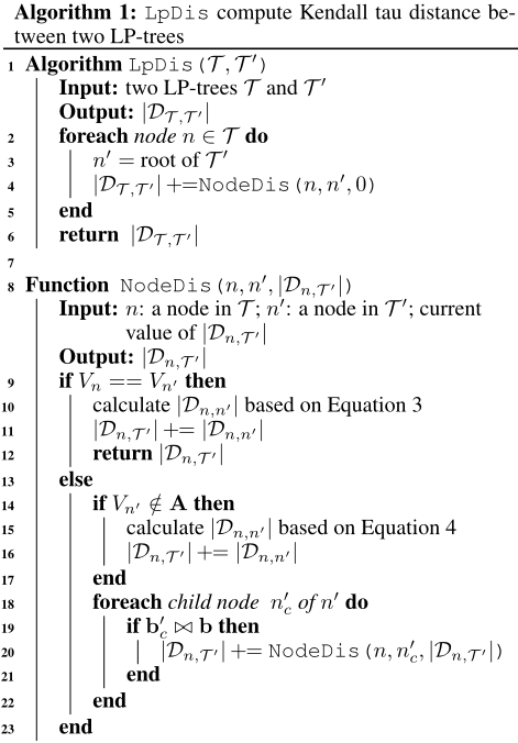
• If n and n′ contain the same attribute Vn == Vn′ (line 9), we calculate the number of disagreement |Dn,n′ | according to Equation 3, add and update the values of |Dn,T ′ | (line 10-11). We then return to the upper-level call and prune the rest of the branch (line 12).
• Otherwise (when Vn ̸= Vn′ ), as mentioned in Section 3.2, if Vn′ is one of the ancestor attributes of Vn in T (Vn′ ∈ A), then Pn ∩ Pn′ = ∅ and |Dn,n′ | = 0. Therefore, we only compute |Dn,n′ | if Vn′ ̸∈ A (line 14). In that case, we calculate |Dn,n′ | based on Equation 4, then add and update the value of |Dn,T ′ | (line 15-16). Note that we will always have Vn /∈ A′ as we stop traversing T ′ and return to the upper level call when Vn == Vn′ , as mentioned in the previous bullet point.

After that, we continue to expand child branches from n′ . For each child node n′c , we examine whether the branching constraint b′c of n′c is consistent with that of n (i.e., b). Conflicting branches are pruned, and for each consistent branch n′c , we call NodeDis with n, n′c and the updated value of |Dn,T ′ | (line 18 - 22).

After ending all recursive calls, NodeDis returns |Dn,T ′ | to its parent function LpDis. We then add |Dn,T ′ | to |DT ,T ′ | (line 4). After repeating it for each node in T , LpDis then returns |DT ,T ′ | as the final output (line 6).

Theorem 1. The proposed LpDis algorithm is complete,

̄

i.e., the final output is equal to the total number of disagreed outcome pairs between T and T ′ .

Proof. During the execution of LpDis, we cover every node n in T . For each node n we traverse every node n′ in T ′ and accumulate |Dn,n′ |, except the followings:

• If Vn = Vn′ , we prune all child branches from n′ . In this case, for any child n′c of n′ , we will have Vn (= Vn′ ) as an ancestor attribute of n′c in T ′ . As discussed in Section 3.2, Pn ∩ Pn′c = ∅ and ∣∣Dn,n′c ∣∣ = 0.
• Similarly, if Vn′ is an ancestor of Vn in T , we do not consider |Dn,n′ |, as Pn ∩ Pn′ = ∅ and |Dn,n′ | = 0.
• If a child node n′c of n′ conflicts with the branching constraints of n, as also discussed in Section 3.2 we will also have Pn ∩ Pn′ = ∅ and |Dn,n′ | = 0.

In other words, for all possible prunings occur in LpDis, we prove that |Dn,n′ | = 0. And therefore, the final returned

Theorem 2. The computation time of the proposed LpDis algorithm is polynomial, quadratic, in the size of the input, i.e., the size of the two LP-trees.

Proof. For a node n in an LP-tree T , let dn be the domain size of Vn and pn be the number of rows in the CPT of n. We can consider the size of an LP-tree as the sum

̄

̄

̄

̄

̄

̄

̄

̄

̄

̄

̄

of the sizes of the CPT on each node of the LP-tree. Assume an LP-tree T has j nodes and T ′ has k nodes, we denote s (resp. s′ ) as the size of T (resp. T ′ ), then s = ∏ i∈{1,··· ,j} dni pni and s′ = ∏ i∈{1,··· ,k} dn′i pn′i . During the exe-

cution of LpDis, we do a nested tree traverse of T and T ′ , so the running time of node visiting is j · k. For each pair of nodes n and n′ when Vn ̸= Vn′ , we can directly calculate |Dn,n′ | with Equation 4. Otherwise, if Vn = Vn′ , we will have to count the number of pairwise disagreements on attribute values in every possible joint parent context, the worst case running time is dnpn · dn′pn′ . Therefore, the worst case complexity of LpDis is O(j · k · dnpn · dn′pn′) = O(j · dnpn · k · dn′pn′) = O(s · s′ ).

Essentially, the running time of LpDis depends on the complexity of the LP-trees, i.e., whether they have complex importance structures (with many different branches), and whether the preference on an attribute depends on many other attributes. In the worst case, the number of nodes in an LPtree and the number of parent context of an attribute grow exponentially in the number of attributes. In which case, however, it is not meaningful to use LP-trees to represent agents' preferences as it constructs a full tree. This is then equivalent to giving out the full ranking over the alternative space.

4.1 Illustration

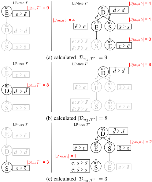
We now demonstrate the execution of LpDis with the two LP-trees T (Figure 1a) and T ′ (Figure 1b). LpDis traverses T , calculates and accumulates |Dn,T ′ | for every node n. Figure 2 shows the calculation for each node.

For n1 in T (Figure 2a), Vn1 = E, we depth-first traverse

• T ′ :· Starting from n′1 in T ′ , as demonstrated in Example 5, ∣∣Dn1,n′1 ∣∣ = 4. We update the value of |Dn1,T ′ | as 0 + ∣∣Dn1,n′1 ∣∣ = 4. Since there is no branching constraint for n1 in T , all child branches of n′1 are consistent with n1. Therefore, we proceed to each child of n′1 .
• We now reach n′2 in T ′ . As Vn′2 = E = Vn1 , we calculate ∣∣Dn1,n′2 ∣∣ based on Equation 3. For n1: A = B = P = ∅, and for n′2 : A′ = B′ = {D}, P = ∅, so ˘A = ˘B = {D}, ˘b = d and ˘P = ∅. Referring to the CPT of n1 and n′2 : e ≻n1 ¯ e, however, ¯ e ≻n′2 e. Hence, the number of disagreed pairwise preference on values of Vn1 (= Vn′2 ) is |ℓ| = 1. Therefore: ∣∣Dn1,n′2 ∣∣ = 1× ∏ X∈∅ |DX| × ∏ Y ∈V\({D}∪{E}) (|DY |)2 =

We subsequently end the current recursive call, return to the parent node n′1 without visiting n′3 , and proceed to another call with parameters n1, child node n′4 , and the current value |Dn1,T | = 4 + ∣∣Dn1,n′2 ∣∣ = 8.

• Similarly for n′4 , Vn′4 = S ̸= Vn1 , ˘A = ˘B = {D}, therefore, according to Equation 4, ∣∣Dn1,n′4 ∣∣ = 1, and the current value |Dn1,T | = 8 + ∣∣Dn1,n′4 ∣∣ = 9.
• At the end, we reach the leaf node n′5 , where Vn′5 = E = Vn. As they both have the same local preference on E (e ≻ ¯ e), therefore, |ℓ| = 0 and ∣∣Dn1,n′5 ∣∣ = 0

After that, NodeDis returns to its parent function LpDis with |Dn1,T ′ | = 9. We then update |DT ,T ′ | = |Dn1,T ′ | = 9. We then move to n2 in T , and depth-first traverse T ′ (see Figure 2b). Right on the root node n′1 , as Vn2 = Vn′1 = D, ˘A = {E}, ˘B = ˘P = ∅, and |ℓ| = 1 (d ≻n2 ¯ d but ¯ d ≻n′1 d), we have ∣∣Dn2,n′1 ∣∣ = 1 × 2 × 22 = 8 (according to Equation 3). We then directly return to LpDis with |Dn2,T ′ | = ∣∣Dn2,n′1 ∣∣ = 8, and update |DT ,T ′ | = 9+ |Dn2,T ′ | = 9+8 = 17. All child branches of n′1 in T ′ are pruned in this iteration.

Lastly, for n3 in T (Figure 2c), we depth-first traverse T ′ :

• On n′1 , Vn′1 = D is an ancestor attribute of n3 in T , we proceed to its child nodes without any computation.
• Similarly on n′2 , as Vn′2 = E is an ancestor attribute of n3 in T , we proceed to the next call to the leaf node n′3 .
• On n′3 , as shown previously in Example 4, we have ∣∣Dn3,n′3 ∣∣ = 1. We update |Dn3,T ′ | = 0 + 1 = 1. Then, we return to n′2 , and subsequently return to n′1 and further proceed to its right child n′4 .
• On n′4 , Vn′4 = Vn3 = S, ˘A = {E,D}, ˘B = {D}, and |ℓ| = 1. According to Equation 3, ∣∣Dn3,n′4 ∣∣ = 1 × 2 × 1 = 2. So |Dn3,T ′ | = 1 + ∣∣Dn3,n′4 ∣∣ = 3. It then prunes the rest of the branch and return to n′1 . NodeDis then returns to LpDis with |Dn3,T ′ | = 3

After that, |DT ,T ′ | = 17 + |Dn3,T ′ | = 20. Now, we have completed the traverse of T and LpDis returns |DT ,T ′ | = 20 as the Kendall tau distance between T and T ′ .

5 Experiments

We compare the proposed approach with a baseline technique called Exhau which performs an exhaustive query over all possible outcome pairs. We generate random LP-trees by varying the number of attributes, the structure of the trees, and the local attribute preferences.

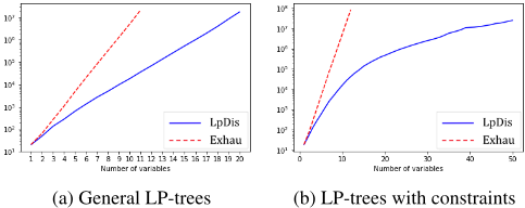
In the first set of experiments, we consider N (number of variables) between 1 to 20 and run 1000 experiments on each number of attributes. All variables are binary. Figure 3a plots the average time spent by these algorithms against the number of attributes. We can see that LpDis runs significantly faster than the Exhau algorithm. As the number of attributes grows the gap between LpDis and Exhau increases. When N = 10, LpDis performs 1000 times faster than Exhau. While it is infeasible to run large-scale experiments with Exhau when the number of variables is more than 11, on average, LpDis runs on 20 attributes in about 15 seconds.

In the second set of experiments, we limit the maximum number of parents of each attribute to 5, and the maximum number of nodes in an LP-tree to be the square of the number of attributes (N 2 ). The results are shown in Figure 3b. In this case, LpDis presents only a polynomial growth on the number of attributes. It runs on 50 attributes in about 25 seconds. In contrast, Exhau does not show any noticeable improvements even after introducing the constraints.

6 Conclusion and FutureWork

We investigated the problem of computing the number of pairwise disagreements (Kendall tau distance) between two agents' preferences represented by LP-trees. We proposed an algorithm called LpDis to calculate such distance with any classes of LP-trees, where the agents do not necessarily share common preference dependencies or attribute importance structures. LpDis retains the accuracy, yet efficiently computes the Kendall tau distance by traversing the LP-trees without generating or querying any outcome pair. As demonstrated with experiments, the improvement in running time compared to the exhaustive querying method is significant.

This research opens up a couple of interesting topics for future exploration, including but not limited to: i) extension for incomplete LP-trees, where some of the attributes are missing in the LP-tree branches, or some of the conditional preference tables (CPTs) on the nodes of the LP-tree are incomplete. While in this work we assume the LP-trees are complete, human preferences in real-world are often incomplete, and possibly inconsistent. We intend to extend the current formulation to accommodate incomplete and/or inconsistent LP-trees. ii) various ML tasks on LP-trees. It would be interesting to cluster or predict agents' preferences by having LPtrees as training samples. We also plan to apply LP-trees in label ranking problem, to discover common decision-making patterns in a group of agents.