
An Exact Algorithm for Maximum k-Plexes in Massive Graphs
Proceedings of the Twenty-Seventh International Joint Conference on Artificial Intelligence. Main track. Pages 1449-1455.
https://doi.org/10.24963/ijcai.2018/201
Keywords
- Heuristic Search and Game Playing: Heuristic Search
- Heuristic Search and Game Playing: Combinatorial Search and Optimisation
Abstract
The maximum k-plex, a generalization of maximum clique, is used to cope with a great number of real-world problems. The aim of this paper is to propose a novel exact k-plex algorithm that can deal with large-scaled graphs with millions of vertices and edges. Specifically, we first propose several new graph reduction methods through a careful analyzing of structures of induced subgraphs. Afterwards, we present a preprocessing method to simplify initial graphs. Additionally, we present a branch-and-bound algorithm integrating the reduction methods as well as a new dynamic vertex selection mechanism. We perform intensive experiments to evaluate our algorithm, and show that the proposed strategies are effective and our algorithm outperforms state-of-the-art algorithms, especially for real-world massive graphs.
- [Balasundaram et al., 2011] Balabhaskar Balasundaram, Sergiy Butenko, and Illya V Hicks. Clique relaxations in social network analysis: The maximum k-plex problem. Operations Research, 59(1):133-142, 2011.
- [Batsyn et al., 2014] Mikhail Batsyn, Boris Goldengorin, Evgeny Maslov, and Panos M. Pardalos. Improvements to MCS algorithm for the maximum clique problem. J. Comb. Optim., 27(2):397-416, 2014.
- [Berlowitz et al., 2015] Devora Berlowitz, Sara Cohen, and Benny Kimelfeld. Efficient enumeration of maximal k- plexes. In Timos K. Sellis, Susan B. Davidson, and Zachary G. Ives, editors, Proceedings of the 2015 ACM SIGMOD International Conference on Management of Data, Melbourne, Victoria, Australia, May 31 -June 4, 2015, pages 431-444. ACM, 2015.
- [Cai and Lin, 2016] Shaowei Cai and Jinkun Lin. Fast solv- ing maximum weight clique problem in massive graphs. In Proceedings of the Twenty-Fifth International Joint Con- ference on Artificial Intelligence, New York, NY, USA, 9-15 July 2016, pages 568-574. IJCAI/AAAI Press, 2016. IJCAI
- [Cai, 2015] Shaowei Cai. Balance between complexity and quality: Local search for minimum vertex cover in mas- sive graphs. In Proceedings of the Twenty-Fourth Inter- national Joint Conference on Artificial Intelligence, IJCAI 2015, Buenos Aires, Argentina, July 25-31, 2015, pages 747-753. AAAI Press, 2015. IJCAI
- [Conte et al., 2016] Alessio Conte, Roberto De Virgilio, An- tonio Maccioni, Maurizio Patrignani, and Riccardo Tor- lone. Finding all maximal cliques in very large social networks. In Proceedings of the 19th International Con- ference on Extending Database Technology, Bordeaux, France, March 15-16, 2016., pages 173-184, 2016.
- [Conte et al., 2017] Alessio Conte, Donatella Firmani, Cate- rina Mordente, Maurizio Patrignani, and Riccardo Tor- lone. Fast enumeration of large k-plexes. In Proceed- ings of the 23rd ACM SIGKDD International Conference on Knowledge Discovery and Data Mining, Halifax, NS, Canada, August 13 -17, 2017, pages 115-124, 2017.
- [Jiang et al., 2017] Hua Jiang, Chu-Min Li, and Felip Manyà. An exact algorithm for the maximum weight clique problem in large graphs. In Proceedings of the Thirty-First AAAI Conference on Artificial Intelligence, February 4-9, 2017, San Francisco, California, USA., pages 830-838, 2017.
- [Lakhlef, 2015] Hicham Lakhlef. A multi-level clustering scheme based on cliques and clusters for wireless sensor networks. Computers & Electrical Engineering, 48:436- 450, 2015.
- [Lin et al., 2017] Jinkun Lin, Shaowei Cai, Chuan Luo, and Kaile Su. A reduction based method for coloring very large graphs. In Proceedings of the Twenty-Sixth Inter- national Joint Conference on Artificial Intelligence, Mel- bourne, Australia, August 19-25, 2017, pages 517-523, 2017. IJCAI
- [Miao and Balasundaram, 2017] Zhuqi Miao and Balab- haskar Balasundaram. Approaches for finding cohesive subgroups in large-scale social networks via maximum k- plex detection. Networks, 69(4):388-407, 2017.
- [Moser et al., 2012] Hannes Moser, Rolf Niedermeier, and Manuel Sorge. Exact combinatorial algorithms and ex- periments for finding maximum k-plexes. Journal of com- binatorial optimization, 24(3):347-373, 2012.
- [Rossi and Ahmed, 2014] Ryan A Rossi and Nesreen K Ahmed. Coloring large complex networks. Social Net- work Analysis and Mining, 4(1):228, 2014.
- [Rossi and Ahmed, 2015] Ryan A. Rossi and Nesreen K. Ahmed. The network data repository with interactive graph analytics and visualization. In Proceedings of the Twenty-Ninth AAAI Conference on Artificial Intelligence, January 25-30, 2015, Austin, Texas, USA., pages 4292- 4293, 2015.
- [Rossi et al., 2014] Ryan A. Rossi, David F. Gleich, Asse- faw Hadish Gebremedhin, and Md. Mostofa Ali Patwary. Fast maximum clique algorithms for large graphs. In Chin- Wan Chung, Andrei Z. Broder, Kyuseok Shim, and Torsten Suel, editors, 23rd International World Wide Web Confer- ence, WWW '14, Seoul, Republic of Korea, April 7-11, 2014, Companion Volume, pages 365-366. ACM, 2014.
- [Seidman and Foster, 1978] Stephen B Seidman and Brian L Foster. A graph-theoretic generalization of the clique con- cept. Journal of Mathematical sociology, 6(1):139-154, 1978.
- [Xiao et al., 2017] Mingyu Xiao, Weibo Lin, Yuanshun Dai, and Yifeng Zeng. A fast algorithm to compute maxi- mum k-plexes in social network analysis. In Proceedings of the Thirty-First AAAI Conference on Artificial Intelli- gence, February 4-9, 2017, San Francisco, California, US- A., pages 919-925, 2017.
- [Zhou and Hao, 2017] Yi Zhou and Jin-Kao Hao. Frequency-driven tabu search for the maximum s- plex problem. Computers & Operations Research, 86:65-78, 2017.
References were extracted automatically from the PDF and may contain errors.
Full text extracted automatically from the PDF; figures, tables and equations may differ. The PDF is the version of record.
1 Introduction
With rapid growth of the information technology, real-world graphs have been growing quickly in the past decade. A significant challenge rises: traditional algorithms fail to deal with newly emerged massive graphs. Therefore, algorithms in massive graphs (or complex networks) have received much attention due to their great importance in real-world applications. There has been a huge amount of efforts devoted to solve various problems, such as maximum cliques [Batsyn et al., 2014; Cai and Lin, 2016], and graph coloring [Rossi and Ahmed, 2014]. Among those problems, the maximum clique can settle various applications [Lakhlef, 2015; Conte et al., 2016].
Due to the strict restrictions of cliques, it is always difficult to model problems directly, so the k-plex was proposed and investigated [Seidman and Foster, 1978; Balasundaram et al., 2011; Conte et al., 2017]. Unlike cliques that restrict a vertex should connect with all other vertices, the k-plex allows every vertex has several missing connections, and thus it is more useful than the clique. Recently, the k-plex has revealed great success in the social network detection [Xiao et al., 2017; Miao and Balasundaram, 2017]. To solve the maximum k-plex, several algorithms were developed, including exact algorithms [Balasundaram et al., 2011; Moser et al., 2012] as well as heuristic methods [Zhou and Hao, 2017]. Moreover, enumeration algorithms for finding all maximal k-plexes larger than a predefined integer were also developed [Berlowitz et al., 2015; Conte et al., 2017]. In recent years, massive graphs have attracted much attention. There are many maximum clique algorithms aiming at massive graphs [Jiang et al., 2017; Cai and Lin, 2016; Rossi et al., 2014]. For example, Jiang et al. [2017] proposed an exact algorithm able to deal with very large garphs. But we have reviewed much fewer algorithms for the maximum k-plex. This is partially because the k-plex is more difficult to solve than cliques due to the relaxation. Among maximum k-plex algorithms, we highlight an exact algorithm proposed by Xiao et al. [2017] very recently, which breaks the trivial exponential bound of 2n for k ≥ 3 and solves graphs containing 10 thousand vertices.
∗ corresponding author
However, real-world graphs have grown extremely large in recent applications. The graphs may include millions of vertices and millions of edges. Those graphs are usually sparse and the degrees follow a power-law distribution. In this paper, we propose an exact algorithm to solve the maximum k-plex problem in massive sparse graphs. The algorithm is based on the framework of the branch-and-bound search and integrated with graph reduction methods and heuristic strategies. First, three reduction methods based on the lower bound are introduced, two of which are particularly developed for sparse graphs through a deep analysis of the structure of induced subgraphs. Moreover, a reduction method using the parameter k is also discussed as a further enhancement. Combinations of these methods are employed in two types of branches, i.e., selecting or discarding a vertex, to reduce search space. Also, reduction methods are performed in the preprocessing so as to simplify initial graphs. In addition, we employ heuristic methods to implement the dynamic vertex selection with the purpose of making the remaining graph as small as possible. Intensive experiments are performed on real-world graphs from Network Data Repository online [Rossi and Ahmed, 2015] and DIMACS benchmarks. First, it shows graphs can be reduced greatly through our preprocessing method. Also, comparative results are analyzed with varying k from 2 to 5, showing that our new algorithm solves graphs up to millions of vertices efficiently and outperforms the existing exact algorithms proposed recently. Finally, we give some conclusions.
2 Preliminaries
Graphs discussed in this paper are simple and undirected. Formally, an undirected graph is defined as G = (V,E), where V is a set of vertices and E is a set of edges. An edge in E is associated with two vertices in V , so an unordered pair of two vertices specifies an edge. We say a vertex u is a neighbor of a vertex v if there is an edge (v, u) in E. The set of the neighbors of a vertex v in V is denoted by NG(v). Specially, we define NG(v) as an empty set if v is not in V . The degree of a vertex v is defined as the number of its neighbors, denoted as dG(v) = |NG(v)|. Given a subset S ⊆ V , G[S] = (V ′ , E′ ) is the induced subgraph in G by S if V ′ = S and the edge set E′ consists of all the edges in E whose both vertices are in S.
Given a graph G = (V, E) and a positive integer k, a subset S ⊆ V is a k-plex if the degree of each vertex in the induced subgraph G[S] is at least |S|-k. We say a k-plex is maximal if any other k-plex cannot strictly contain it. The maximum k-plex problem is to find the k-plex with the largest size of a given graph. It is easy to see a 1-plex is a clique. It is proved that finding a k-plex with a fixed size is NP-complete for any constant positive integer k [Balasundaram et al., 2011].
3 Graph Reductions
In this section, we present some new theoretical results useful for graph reductions.
3.1 Properties
The first result is straightforward.
Property 1. Given a graph G = (V, E), and a positive integer LB, a vertex v cannot be included in a k-plex larger than LB if dG(v) + k ≤ LB.
Obviously, Property 1 is correct due to the definition of the k-plex. Such vertex v can be removed from the graph when we search a k-plex larger than LB. However, the effect of this property is limited since it basically relies on vertex degrees.
To reduce more vertices, a complex situation is discussed below. We provide some notions first. Given a graph G = (V,E), a k-plex S ⊆ V , and a vertex u in V , we define the notation rG,S(u) as
It indicates that a maximal k-plex containing S ∪ {u} can further include at most rG,S(u) vertices from V \ (S ∪ {u} ∪ NG(u)). Note that u can be either an element in S or in V \S. The notation cG,S(u, v) is defined as
cG,S(u, v) = min(dG′ (u)+rG,S(u)+1, |V ′ |)+rG,S(v), (2) where G′ (V ′ , E′ ) = G[(NG(v)\S)∪{v}], v is a vertex in V , u is a vertex in V ′ \ {v}, and function min returns the smaller value between two parameters.
Property 2. Given a graph G = (V, E) and a k-plex S ⊆ V , the maximum k-plex including S ∪ {u, v} is no larger than cG,S(u, v) + |S \ {v}|, where v is a vertex in V and u is a vertex in NG(v) \ S.
Proof. Let G′ (V ′ , E′ ) = G[(NG(v) \ S) ∪ {v}]. We divide vertices from V \ S into 2 parts: the first one is V \ (V ′ ∪S), from which we can choose rG,S(v) vertices at most due to the restriction on non-neighbors of v; the second one is V ′ . After u and v are selected, due to the restriction on non-neighbors of u, at most dG′(u) - |{v}| + rG,S(u) extra vertices can be selected in V ′ if there are enough vertices. Otherwise, all vertices in |V ′ | can be selected legally. So min(dG′(u) + rG,S(u)+1, |V ′ |) is an upper bound of the vertices including u and v from V ′ , and thus the the maximum k-plex including S ∪ {u, v} is no larger than cG,S(u, v) + |S \ {v}|.
Property 3. Given a graph G = (V, E), a k-plex S ⊆ V , a vertex v in S, and a vertex u in NG(v) \ S, S ∪ {u} cannot be involved in a k-plex larger than a positive integer LB if cG,S(u, v) + |S| - 1 ≤ LB.
It is easy to see Property 3 is correct according to Property 2. Furthermore, we can also apply Property 2 to make a further reduction. When we try to add a vertex v into S, we can check each vertex u in G′ = G[(NG(v) \ S) ∪ {v}], and remove the vertex u (u ̸= v) satisfying Property 2 under a given lower bound LB temporarily. We use V ∗ to denote the remaining vertex set of G′ . After that, we can count the vertices in V ∗ to determine whether v can be removed or added into S. Thereafter, we have the following property.
Property 4. Given a graph G=(V, E), a k-plex S ⊆ V and a vertex v in V \ S, S ∪ {v} cannot be included in a k-plex larger than a positive integer LB if there exists a remaining vertex set V ∗ such that |S| + |V ∗ | + rG,S(v) ≤ LB.
Proof. It is obvious that we can choose at most rG,S(v) vertices from V \ (S ∪ V ∗ ). With the case that all vertices in V ∗ can be selected, we obtain |S| + |V ∗ | + rG,S(v) as an upper bound of the k-plex. Thereafter, v cannot be included in a k-plex larger than LB.
To explain Property 4, we provide an example shown in Figure 1, where S = {s1}. Then we check v, and have G′ = G[(NG(v) \ S) ∪ {v}] composed of u, v and w3. In the case k = 2 and LB = 4, we have rG,S(v) = 1, rG,S(u) = 0 and dG′(u) = 1, and thus cG,S(u, v) + |S| = 4 equal to LB. Therefore, u is removed from G′ temporarily, and thus V ∗ = {v, w3}. Then, we have |S| + |V ∗ | + rG,S(v) = 4, so v should be removed when searching a k-plex larger than 4.
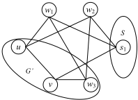
Property 4 is useful for further reduction on remaining vertices that cannot be deleted by Property 1. The sparser the graph is, the more vertices in the induced graph can be deleted. Therefore, efforts will be promoted for sparse graphs.
3.2 Graph Reduction Algorithms
With the graph reduction properties presented above, we propose several reduction algorithms. The first one, we call vertex-reduction, is based on Property 1. The detailed description of vertex-reduction is shown in Algorithm 1.
Algorithm 1: function vertex-reduction(G, LB, k)
Input: G = (V, E), k the k-plex parameter, LB a lower bound Output: G the reduced graph 1 Q← ∅; 2 foreach vertex v in V do 3 if dG(v) + k ≤ LB then add v into Q; 4 while Q is not empty do 5 v ← pop a vertex in Q; 6 foreach u in NG(v) do 7 if dG(u) + k - 1 ≤ LB then add u into Q; 8 if v is in V then remove v fromG; 9 return G;The second one employs Property 4 to reduce the graph by counting allowed vertices in induced subgraphs, so we call it subgraph-reduction, shown in Algorithm 2. Rather than vertex-reduction that reduces the graph to minimal, subgraphreduction only checks each vertex once. When it finds a vertex that can be removed, it reduces the graph and updates vertex degrees immediately and then checks the next vertex. Subgraph-reduction runs in O(|V |×(|V |+|E|)) time, so the efficiency may be increased if the graph is sparse.
Algorithm 2: function subgraph-reduction(G, S, LB, k, C)
Input: G = (V, E), S a k-plex in G (S ⊆ V ), k the k-plex parameter, LB a lower bound, C the vertex set to be checked satisfying C ∩ S = ∅ Output: G the reduced graph 1 foreach vertex v in C do 2 compute rG,S(u) by Eq. (1), for ∀u ∈ (NG(v) \ S) ∪ {v}; 3 G′′ (V ′′ ,E′′ )←G, and Q← ∅; 4 foreach u in NG′′ (v) \ S do 5 compute cG′′,S(u, v) by Eq. (2); 6 if cG′′,S(u, v) ≤ LB-|S| then add u into Q; 7 while Q is not empty do 8 u ← pop a vertex in Q; 9 H ← (NG′′ (u) ∩ NG′′ (v)) \ S; 10 if u is in V ′′ then remove u fromG′′ ; 11 foreach w in H do 12 update cG′′,S(w, v) by Eq. (2) ; 13 if cG′′,S(w, v) ≤ LB-|S| then add w into Q; 14 if |(NG′′ (v) ∪ {v}) \ S| + rG,S(v) ≤ LB-|S| then 15 remove v fromG; 16 break; 17 return G;Similarly, according to Property 3, we present the reduction method called v-reduction in Algorithm 3. It can reduce vertices in the induced subgraph after a vertex v is selected. It works similar to subgraph-reduction, but it removes vertices from G directly, since vertices not satisfying Property 3 no longer makes efforts.
Algorithm 3: function v-reduction(G, S, LB, k, v)
Input: G = (V, E), S a k-plex in G (S ⊆ V ), k the k-plex parameter, LB a lower bound, v a vertex in S Output: G the reduced graph 1 compute rG,S(u) by Eq. (1), for ∀u ∈ (NG(v) \ S) ∪ {v}; 2 Q← ∅; 3 foreach u in NG(v) \ S do 4 compute cG,S(u, v) by Eq. (2); 5 if cG,S(u, v) ≤ LB-|S| + 1 then add u into Q; 6 while Q is not empty do 7 u ←pop a vertex in Q; 8 H ← (NG(u) ∩NG(v)) \ S; 9 if u is in V then remove u fromG; 10 foreach w in H do 11 update cG,S(w, v) by Eq. (2); 12 if cG,S(w, v) ≤ LB-|S| + 1 then add w into Q; 13 return G;Beside those methods, a strategy to deal with vertices violating the k-plex constraint is introduced here. If we aim at finding a k-plex including S, two kinds of vertices should be removed: 1) if there is a vertex u in S satisfying |S \ NG(u)| + 1 = k, then all vertices in V \ (NG(u) ∪ S) should be removed; 2) if there is a vertex u in V \S satisfying |S \NG(u)|+1 > k, then u should be removed. Algorithm 4 formally describes how to reduce the graph using the strategy above.
Algorithm 4: function k-reduction(G, S, k)
Input: G = (V, E), S a k-plex in G (S ⊆ V ), k the k-plex parameter, LB a lower bound Output: G the reduced graph 1 foreach u in S satisfying |S \NG(u)| +1 = k do 2 remove any w in V \ (NG(u) ∪ S) from G; 3 foreach u in V \ S satisfying |S \NG(u)| +1 > k do 4 remove u from G; 5 return G;4 Preprocessing
As we know, massive graphs may have numerous nodes, which may cause the execution of an algorithm out of memory. So preprocessing is a necessary step, which can usually reduce the input graphs to a reasonable size. The more nodes in the original graphs are removed, the less branches are exploited in the searching algorithm. Algorithm 5 shows the procedure of the preprocessing step. We employ a heuristic method to obtain a lower bound, which is an extension of the method in [Jiang et al., 2017]. Based on the lower bound, vertex-reduction can reduce graphs efficiently due to its linear computation time for checking a vertex. However, the effectiveness, unfortunately, is not satisfactory, if the heuristic method fails to find a lower bound close to the optimal value.
It is not surprise that a heuristic sometimes finds a solution far from the best one. As a result, subgraph-reduction is also used in preprocessing for a further reduction. With the same lower bound, it can remove more vertices, though it needs higher computation complexity. Two reduction methods are preformed alternatively until no vertex can be removed. During iterations, the lower bound is updated before each execution of the vertex-reduction, since the heuristic may find new lower bounds when the graph is reduced.
Algorithm 5: function reduce-graph(G,k)
Input: G = (V, E), k the k-plex parameter. Output: LB a lower bound, and G the reduced graph 1 m ← |V | + 1,LB ← 0; 2 while |V | <mdo 3 m← |V |; 4 if LB-heuristic(G, k) > LB then 5 LB ← LB-heuristic(G, k); 6 G←vertex-reduction(G,LB, k); 7 G← subgraph-reduction(G, ∅,LB, k, V ); 8 return (LB, G); 9 function LB-heuristic(G, k); 10 for i ← 1 to |V | do 11 v ← the vertex with the smallest dG(v) in V ; 12 if dG(v) + k ≥ |V | then break; 13 remove v fromG; 14 return |V |;5 The Branch-and-Bound Algorithm
In this section, we present our branch-and-bound algorithm. The entire framework of the algorithm is indicated in Algorithm 6.
The algorithm starts with the preprocessing algorithm to reduce the input graphs, and then it performs the branch-andbound algorithm. Search tree nodes are expanded recursively by the function BB. It returns the size of S if there is no vertex left, or the best lower bound found in its branch. There are some crucial components in the function BB to be explained.
The first one is the reduction methods. The branching rule here is binary, i.e., selecting a vertex and adding it into the target k-plex or discarding the vertex. After that, reductions are performed to simplify the remaining graph. Two combinations of reduction methods are employed after selecting and discarding, respectively.
In a selecting branch, we take three reduction methods. They are performed in the ordering of k-reduction, vertexreduction and v-reduction. The reason of taking this ordering is under the following observation: vertex-reduction cannot make efforts if performed first as it is irrelevant with S, but k-reduction can delete all conflict vertices directly. Therefore k-reduction is the first, and then vertex-reduction and v-reduction. Different from the preprocessing step, vreduction is employed instead of the subgraph-reduction due to the efficiency. In a discarding branch, vertex-reduction and subgraph-reduction are used. Obviously, k-reduction
Input: G = (V, E), k the k-plex parameter. Output: the size of the maximum k-plex 1 S ← ∅; 2 (LB,G) ← reduce-graph(G, k); 3 LB ←BB(G, S, k,LB); 4 return LB; 5 function BB(G, S, k,LB); 6 if V \ S is empty then return |S|; 7 select a vertex v in V \ S, and S ← S ∪ {v}; 8 store G as Gr; 9 G←k-reduction(G, S, k); 10 G←vertex-reduction(G,LB, k); 11 G←v-reduction(G, S,LB, k, v); 12 if |{u|u in V \ S and dG(u) +k > LB}| + |S| > LB then 13 lower ← BB(G, S, k, LB); 14 if LB < lower then LB ← lower; 15 restore Gr to G; 16 S ← S \ {v}, and remove v from G; 17 G←vertex-reduction(G,LB, k); 18 G← subgraph-reduction(G, S,LB, k, V \ S); 19 if |{u|u in V \ S and dG(u) +k > LB}| + |S| > LB then 20 lower ← BB(G, S, k, LB); 21 if LB < lower then LB ← lower; 22 return LB;could not work in this branch, since S does not change after discarding a vertex so as to rG,S(v). However, the fact that degrees of discarded vertex's neighbors decrease makes vertex-reduction work well. To further enhance the reduction, subgraph-reduction is performed after vertex-reduction. Different from reducing graphs iteratively, all reductions are performed only once after selecting or discarding.
The second component discussed is the computation of upper bounds. After reductions, the algorithm should compute upper bounds to determine selecting a new vertex or trying another branch. Since the graph is reduced deeply, a simple but efficient method that counts the number of remaining vertices is developed for the upper bound, but the actual number of remaining vertices is not used as the bound directly in our algorithm. This is because the reduction methods during branch-and-bound searching are not performed iteratively, as we described above, and thus some vertices in a reduced graph may still satisfy the vertex-reduction rule. Therefore, we have to scan the vertices again to calculate the bound. To speed up this task, we employ a lazy method to determine whether the current branch has an upper bound bigger than the lower bound, rather than the method computing the exact value of the upper bound. This is achieved by counting remaining vertex whose degree exceeds the lower bound plus k. If it finds more than LB such vertices, the algorithm executes the function BB; otherwise, it tries the other branch or backtracks to the previous level.
The last one is the vertex selection heuristic, which specifies how to select a vertex on each node of the search tree. As we know the ordering of vertex selection may impact greatly on the search tree size. To make the selection mechanism effective, a dynamic vertex ordering strategy is employed in our algorithm. It selects a vertex according to the current branch and the remaining graph. The purpose of the dynamic vertex ordering strategy is to delete vertices as many as possible in the reduction after a selection. As the reduction algorithms are mainly based on vertex degrees, it is clear that selecting the vertex with the maximum degree from the remaining graph is a basic strategy that can decrease vertex degrees in full measure. Furthermore, our reduction method k-reduction is according to the value rG,S(v), the maximal allowed nonneighbors from the remaining graph, and thus if a vertex v with rG,S(v) = 0 is selected, all its non-neighbors can be removed. So a compound measurement is proposed, where rG,S(v) = 0 is the primary condition while the degree is the secondary condition used to break ties.
With the discussion above, two ordering rules are considered in our algorithm.
Rule 1. Select the vertex v with the maximum dG[V \S](v).
Rule 2. Select the vertex v with the maximum dG[V \S](v) from V0 = {v|k = |S\NG(v)|+1} if V0 is not empty; Select the vertex according to Rule 1 otherwise.
If there is more than one vertex as candidates, select the first one in lexicographical order. We call the BnB with Rule 1 as the vertex selection strategy BnBd, and the BnB with Rule 2 BnBk. In the following section, we will show comparative results of the exact algorithm we proposed.
6 Experiments
In this section, we performed intensive experiments to evaluate the algorithm we proposed. Two benchmarks were considered. One is selected instances from DIMACS benchmark, tested in [Xiao et al., 2017]. The other is real-world massive graphs, originally from the Network Data Repository online [Rossi and Ahmed, 2015], where 139 massive sparse graphs are selected 1 . Those benchmarks are popular on evaluating various massive graph algorithms [Rossi and Ahmed, 2014; Cai, 2015; Lin et al., 2017].
Our algorithms were implemented in C++ language and compiled by g++ version 4.7 with -O3 option. Benchmarks were solved parallel on a workstation with an Intel Xeon E5-1650v4 (3.6GHz) CPU, and 16GB RAM, running Ubuntu Linux 16.04, with the cutoff time 10000s. There are several exact algorithms proposed for the maximum k-plex, such as IPBC [Balasundaram et al., 2011], GuidedBranching [Moser et al., 2012] and BS [Xiao et al., 2017].
We first compare our algorithms with the three algorithms on DIMACS benchmarks fixing k = 2. Table 1 indicates runtimes, where "-" means time out or out of memory. BS and our algorithms are computed by our workstation whereas data of others come from [Xiao et al., 2017], which were computed by slower machines. From Table 1, it can be seen that IPBC is faster than others on hamming and johson instances, but those instances are relatively small. BS, BnBd and BnBk are good at solving instances with more than 200 vertices, such as c-fat500, brock and p hat instances. This result is compatible with [Xiao et al., 2017], in which it is reported that BS outperforms others on large instances (e.g. social networks). Among BS, BnBd and BnBk, BnBk performs best on most instances.
1 available at: http://lcs.ios.ac.cn/˜caisw/Resource/realworld%20 graphs.tar.gz
| instance | IPBC | GuideBranching | BS | BnBd | BnBk |
|---|---|---|---|---|---|
| c-fat200-1 | 148.9 | 1.1 | 0.112 | 0.008 | 0.004 |
| c-fat200-2 | 19.1 | 3.53 | 0.132 | 0.004 | 0 |
| c-fat200-5 | 2.1 | 22.44 | 0.158 | 0.036 | 0.028 |
| c-fat500-1 | 1356 | 11.01 | 0.408 | 0.008 | 0.016 |
| c-fat500-2 | 605.3 | 50.21 | 0.536 | 0.068 | 0.024 |
| c-fat500-5 | 141.5 | 350.6 | 0.352 | 0.132 | 0.108 |
| c-fat500-10 | 76.5 | 1547 | 0.47 | 0.388 | 0.424 |
| hamming6-2 | 0 | 1.77 | 32.59 | 110.9 | 13.82 |
| hamming6-4 | 0.3 | 0.24 | 0.066 | 0.024 | 0.02 |
| hamming8-4 | 8115 | - | - | - | - |
| johnson8-2-4 | 0 | 0.02 | 0.012 | 0.008 | 0.004 |
| johnson8-4-4 | 4.4 | 40.7 | 228.9 | 20.92 | 8.836 |
| MANN a9 | 0 | 0.09 | 4.218 | 16.66 | 11.26 |
| brock200 2 | - | 606.1 | 409.8 | 268.7 | 55 |
| brock200 4 | - | 9691 | - | - | 4121 |
| p hat300-1 | - | 502.5 | 31.84 | 12.91 | 9.368 |
| p hat700-1 | - | - | - | 5527 | 1970 |
Consequently, we compare our algorithms with BS on massive graphs in the followings. It is noted that benchmarks from the Network Data Repository online includes many graphs with millions of vertices, which are much larger than the social networks (10 thousand vertices at maximum) used in [Xiao et al., 2017].
Before analyzing runtimes on massive graphs, we show the effect made by our subgraph-reduction. We count the remaining vertices in the preprocessing step compared to the method with vertex-reduction only (removing subgraphreduction from function reduce-graph). Detailed results of the facebook networks with k = 2 and k = 5 are listed in Table 2. It shows that using subgraph-reduction can remove much more vertices compared with using vertex-reduction only. In fact, the preprocessing function reduce-graph can reduce to 0.15% scale of the original graphs on average of 139 instances when k = 2, about 1/20 size of the vertex-reduction results. Surprisingly, it can reduce 68 out of 139 graphs to empty and thus achieved the maximum solutions without the branch-and-bound search. Moreover, similar results can be achieved when k =3,4,5.
| original | k = 2 | k = 5 | |||
|---|---|---|---|---|---|
| networks | size | vertex reduction | reduce- graph | vertex reduction | reduce- graph |
| socfb-A-anon | 3097165 | 390144 | 2239 | 298641 | 819 |
| socfb-B-anon | 2937612 | 489129 | 37564 | 432416 | 34767 |
| socfb-Berkeley13 | 22900 | 12322 | 831 | 10136 | 292 |
| socfb-CMU | 6621 | 3616 | 289 | 3209 | 54 |
| socfb-Duke14 | 9885 | 7090 | 685 | 6536 | 399 |
| socfb-Indiana | 29732 | 19088 | 2316 | 15859 | 976 |
| socfb-MIT | 6402 | 3871 | 280 | 3578 | 60 |
| socfb-OR | 63392 | 10506 | 294 | 7599 | 180 |
| socfb-Penn94 | 41536 | 20353 | 0 | 17080 | 59 |
| socfb-Stanford3 | 11586 | 7759 | 3021 | 7109 | 1388 |
| socfb-Texas84 | 36364 | 16086 | 452 | 9918 | 111 |
| socfb-uci-uni | 58790782 | 499697 | 0 | 26159 | 0 |
| socfb-UCLA | 20453 | 7631 | 66 | 6877 | 65 |
| socfb-UConn | 17206 | 4574 | 63 | 899 | 63 |
| socfb-UCSB37 | 14917 | 1050 | 148 | 814 | 0 |
| socfb-UF | 35111 | 14613 | 1527 | 8526 | 714 |
| socfb-Uillinois | 30795 | 24838 | 6629 | 21421 | 3938 |
| socfb-Wisconsin87 | 23831 | 12709 | 266 | 10431 | 132 |
Table 3 indicates statistic results grouped by families with k =2,3,4,5, respectively, by counting the successfully solved instances of three algorithms: BS, BnBk and BnBd. We use family abbreviations in the table, and full names are biological networks, collaboration networks, Facebook networks, interaction networks, infrastructure networks, amazon recommend networks, retweet networks, scientific computation networks, social networks, technological networks, temporal reachability networks and web link networks.
| Families | k = 2 | k = 3 | k = 4 | k = 5 | ||||||||
|---|---|---|---|---|---|---|---|---|---|---|---|---|
| (#instance) | BS | BnBd | BnBk | BS | BnBd | BnBk | BS | BnBd | BnBk | BS | BnBd | BnBk |
| bio (4) | 4 | 4 | 4 | 4 | 4 | 4 | 4 | 4 | 4 | 4 | 4 | 4 |
| col (13) | 12 | 13 | 13 | 12 | 13 | 13 | 12 | 13 | 13 | 12 | 13 | 13 |
| fb (18) | 3 | 15 | 16 | 2 | 14 | 14 | 2 | 14 | 14 | 1 | 15 | 15 |
| inf (4) | 2 | 4 | 4 | 2 | 4 | 4 | 2 | 2 | 2 | 2 | 1 | 1 |
| int (9) | 8 | 9 | 9 | 7 | 9 | 9 | 7 | 9 | 9 | 6 | 9 | 9 |
| rec (1) | 0 | 1 | 1 | 0 | 1 | 1 | 0 | 0 | 0 | 0 | 0 | 0 |
| ret (3) | 2 | 3 | 3 | 2 | 3 | 3 | 2 | 3 | 3 | 2 | 3 | 3 |
| sci (8) | 2 | 5 | 5 | 2 | 2 | 2 | 1 | 1 | 1 | 2 | 1 | 1 |
| soc (23) | 10 | 16 | 17 | 9 | 17 | 18 | 7 | 16 | 16 | 6 | 16 | 16 |
| tec (7) | 7 | 5 | 6 | 6 | 6 | 7 | 4 | 6 | 6 | 4 | 7 | 7 |
| tem (37) | 37 | 37 | 37 | 37 | 37 | 37 | 37 | 36 | 36 | 37 | 35 | 35 |
| web (12) | 12 | 12 | 12 | 11 | 12 | 12 | 11 | 11 | 11 | 11 | 10 | 10 |
| total (139) | 99 | 124 | 127 | 94 | 122 | 124 | 89 | 115 | 115 | 87 | 114 | 114 |
From Table 3, it is easy to see that BnBk solves the most amount of instances among the three algorithms, much more than BS. For each k, BnBk also performs best. Indeed, most instances solved by BS can also be solved by BnBk successfully, except only 7 instances partly due to unsatisfactory lower bounds obtained. In contrast, BS fails to solve some instances that can be solved by BnBk very easily, or saying within 100s. Also, BnBd reveals better performance than BS, but solves a bit fewer instances than BnBk. Moreover, the number of solved instances decreases with k growing for each algorithm, because most instances become harder to solve.
We then analyze runtimes. We only show solved instances with more than 50000 vertices, and thus select out 44 instances. Table 4 indicates runtimes with k=2,5, respectively, where "-" means time out or out of memory. It shows that BnBd and BnBk are much faster than BS on most instances; BnBd is slightly better than BnBk if instances can be solved in a short time; but BnBk shows a distinct advantage when instances are hard to solve, i.e., larger than 100s.
We also compare our BnBk with BS on the reduced instances. Specifically, we reduce benchmark instances with our preprocessing method, and then solve the reduced instances by both algorithms. Runtimes excluding preprocessing time are listed in Table 5, where instances solved within 10s and unsolved instances are omitted. From it, we can see BS is greatly improved when combining our preprocessing method as more instances can be solved than the original BS. Among 27 instances, BnBk performs better on 18 instances whereas BS on 9 instances. In total, BnBk is also better than BS when BS is associated with our preprocessing method.
7 Conclusions
To solve maximum k-plexes exactly, we have proposed a branch-and-bound algorithm for massive sparse graphs.
| k=2 | k=5 | |||||
|---|---|---|---|---|---|---|
| instance | BS | BnBd | BnBk | BS | BnBd | BnBk |
| ca-citeseer | 0.692 | 0.424 | 0.524 | 0.512 | 0.496 | 0.448 |
| ca-coauthors-dblp | 12.41 | 9.064 | 9.6 | 11.34 | 10.65 | 12.75 |
| ca-dblp-2010 | 0.448 | 0.436 | 0.352 | 0.348 | 0.38 | 0.428 |
| ca-dblp-2012 | 1.245 | 0.656 | 0.52 | 0.853 | 0.672 | 0.756 |
| ca-hollywood-2009 | - | 31.59 | 38.86 | - | 34.14 | 37.83 |
| ca-MathSciNet | 0.965 | 0.404 | 0.68 | 0.823 | 0.592 | 0.688 |
| socfb-A-anon | - | 153.2 | 154.9 | - | 207.4 | 180.9 |
| socfb-B-anon | - | 840.1 | 1012 | - | - | - |
| socfb-OR | - | 26.004 | 8.036 | - | 7.7 | 5.276 |
| socfb-uci-uni | - | 86.14 | 112.9 | - | 82.99 | 90.08 |
| inf-roadNet-CA | 8.056 | 1.824 | 2.012 | 8.401 | - | - |
| inf-roadNet-PA | - | 0.988 | 1.044 | - | - | - |
| inf-road-usa | - | 22.2 | 24.42 | - | - | - |
| ia-wiki-Talk | - | 18.09 | 11.85 | - | 2779 | 938.5 |
| rec-amazon | - | 0.112 | 0.072 | - | - | - |
| rt-retweet-crawl | - | 2.536 | 2.664 | - | 2.092 | 2.208 |
| sc-nasasrb | - | 332.1 | 340.4 | - | - | - |
| sc-pkustk11 | - | 3.528 | 3.776 | - | 3838 | 3705 |
| sc-pkustk13 | - | 275.8 | 313.8 | - | - | - |
| sc-shipsec1 | 600.1 | 1.428 | 1.388 | 675.2 | - | - |
| sc-shipsec5 | 1144 | 30.77 | 32.08 | 1064 | - | - |
| soc-brightkite | 1.185 | 0.136 | 0.244 | 345.5 | 0.168 | 0.156 |
| soc-delicious | 43.34 | 1.192 | 1.204 | - | 1.236 | 1.276 |
| soc-douban | 83.29 | 0.352 | 0.572 | 78.09 | 0.376 | 0.384 |
| soc-flixster | - | - | 465.7 | - | - | - |
| soc-FourSquare | - | - | - | - | 411.5 | 395.6 |
| soc-gowalla | - | 24.99 | 11.96 | - | 279.1 | 106.7 |
| soc-lastfm | - | 165.5 | 108.4 | - | 7039 | 1896 |
| soc-livejouranl | 46.44 | 17.43 | 20.01 | 46.23 | 22.21 | 19.91 |
| soc-LiveMocha | - | 313.3 | 220.1 | - | - | - |
| soc-pokec | - | 74.54 | 75.73 | - | 65.99 | 63.64 |
| soc-slashdot | 96.19 | 252.6 | 17.05 | - | 440.1 | 266.8 |
| soc-twitter-follows | 4683 | 4.52 | 4.68 | - | 25.01 | 21.76 |
| soc-youtube | - | 11.01 | 11.65 | - | 212.6 | 109.9 |
| soc-youtube-snap | - | 17.61 | 15.88 | - | 612.1 | 322.7 |
| tech-as-skitter | 3845 | - | 1426 | - | 170.3 | 77.22 |
| tech-p2p-gnutella | 67.23 | 0.084 | 0.108 | 352.2 | 0.1 | 0.092 |
| tech-RL-caida | 68.38 | 1.524 | 1.592 | - | 1.224 | 1.352 |
| scc retweet-crawl | 0.109 | 0.14 | 0.076 | 0.098 | 0.084 | 0.128 |
| web-arabic-2005 | 0.579 | 0.872 | 0.82 | 0.68 | 0.896 | 0.72 |
| web-it-2004 | 76.59 | 8.576 | 9.444 | 77.89 | 2817 | 2859 |
| web-sk-2005 | 0.22 | 0.256 | 0.18 | 0.325 | 16.98 | 17.14 |
| web-uk-2005 | 59.78 | 19.19 | 19.88 | 60.86 | - | - |
| web-wikipedia2009 | 914.2 | 43.29 | 41.7 | - | - | - |
| instance | k=2 | instance | k=2 | ||
|---|---|---|---|---|---|
| BS | BnBk | BS | BnBk | ||
| socfb-A-anon | 1012 | 28.99 | soc-flixster soc-gowalla | 91.80 | 455.0 |
| socfb-B-anon | - | 755.4 | 115.0 | 7.328 | |
| socfb-Duke14 | 958.1 | 841.2 | soc-lastfm | 2663 | 90.68 |
| socfb-Indiana | 565.1 | 417.4 | soc-LiveMocha | - | 179.2 |
| socfb-MIT | 10.72 | 36.52 | soc-slashdot | 6.162 | 16.50 |
| socfb-Stanford3 | 6704 | 179.4 | soc-twitter-follows | 2073 | 1.504 |
| socfb-Texas84 | 108.3 | - | soc-youtube | 158.4 | 3.252 |
| socfb-UF | 584.4 | - | soc-youtube-snap | 782.7 | 5.516 |
| socfb-Uillinois | 2083 | 429.6 | tech-as-skitter | 483.3 | 1414 |
| ia-enron-large | 21.88 | 0.920 | tech-WHOIS | 50.56 | - |
| ia-wiki-Talk | 136.7 | 10.08 | scc fb-forum | 0.180 | 394.0 |
| sc-nasasrb | - | 338.0 | scc twitter-copen | 0.336 | 94.26 |
| sc-pkustk13 | - | 272.9 | web-wikipedia2009 | 764.8 | 35.21 |
| sc-shipsec5 | 148.8 | 29.97 | |||
Three main components have been described in detail. Special graph reduction methods for sparse graphs have been proposed to enhance the efficiency of the algorithm, where analyzing of induced subgraph structures makes significant effects. Moreover, a dynamic vertex selection mechanism has been proposed to speed up searching. Additionally, a lazy computation of the upper bound has been introduced. Besides, a preprocessing method with our reduction strategies has been introduced in the algorithm, which may always reduce massive graphs to tractable sizes. We have shown our reduction strategies work effectively through computational experiments, and our algorithm outperforms the state-of-theart exact algorithms. It is also worth to mention that the graph with more than 50 million vertices can be solved in a very short time by our algorithm. In the future, parallelization of the proposed methods and algorithms for maximum weighted k-plex problems are valuable research directions.
Acknowledgments
We are grateful to the anonymous reviewers for their constructive comments which have helped us to significantly improve the paper. This work was supported by National Natural Science Foundation of China (Grant Nos. 61672122, 61503074, 61402070, 61370156, and 61602077).
@inproceedings{ijcai2018p201,
  title     = {An Exact Algorithm for Maximum k-Plexes in Massive Graphs},
  author    = {Gao, Jian and Chen, Jiejiang and Yin, Minghao and Chen, Rong and Wang, Yiyuan},
  booktitle = {Proceedings of the Twenty-Seventh International Joint Conference on
               Artificial Intelligence, {IJCAI-18}},
  publisher = {International Joint Conferences on Artificial Intelligence Organization},
  editor    = {Jérôme Lang},
  pages     = {1449--1455},
  year      = {2018},
  month     = {7},
  note      = {Main track},
  doi       = {10.24963/ijcai.2018/201},
  url       = {https://doi.org/10.24963/ijcai.2018/201},
}
TY - CPAPER TI - An Exact Algorithm for Maximum k-Plexes in Massive Graphs AU - Gao, Jian AU - Chen, Jiejiang AU - Yin, Minghao AU - Chen, Rong AU - Wang, Yiyuan T2 - Proceedings of the Twenty-Seventh International Joint Conference on Artificial Intelligence, IJCAI-18 PB - International Joint Conferences on Artificial Intelligence Organization PY - 2018 SP - 1449 EP - 1455 DO - 10.24963/ijcai.2018/201 UR - https://doi.org/10.24963/ijcai.2018/201 ER -Copied
Machine-readable versions of this paper, for tools and AI agents:





