
A Reactive Strategy for High-Level Consistency During Search
Proceedings of the Twenty-Seventh International Joint Conference on Artificial Intelligence. Main track. Pages 1390-1397.
https://doi.org/10.24963/ijcai.2018/193
Keywords
- Constraints and SAT: Constraint Satisfaction
- Constraints and SAT: Constraints: Solvers and Tools
Abstract
Constraint propagation during backtrack search significantly improves the performance of solving a Constraint Satisfaction Problem. While Generalized Arc Consistency (GAC) is the most popular level of propagation, higher-level consistencies (HLC) are needed to solve difficult instances. Deciding to enforce an HLC instead of GAC remains the topic of active research. We propose a simple and effective strategy that reactively triggers an HLC by monitoring search performance: When search starts thrashing, we trigger an HLC, then conservatively revert to GAC. We detect thrashing by counting the number of backtracks at each level of the search tree and geometrically adjust the frequency of triggering an HLC based on its filtering effectiveness. We validate our approach on benchmark problems using Partition-One Arc-Consistency as an HLC. However, our strategy is generic and can be used with other higher-level consistency algorithms.
- [Balafrej et al., 2013] Amine Balafrej, Christian Bessiere, Remi Coletta, and El-Houssine Bouyakhf. Adaptive Pa- rameterized Consistency. In Proc. of CP'13, volume 8124 of LNCS, pages 143-158. Springer, 2013.
- [Balafrej et al., 2014] Amine Balafrej, Christian Bessiere, El-Houssine Bouyakhf, and Gilles Trombettoni. Adaptive Singleton-Based Consistencies. In Proc. of AAAI-2014, pages 2601-2607, 2014.
- [Balafrej et al., 2015] Amine Balafrej, Christian Bessière, and Anastasia Paparrizou. Multi-Armed Bandits for Adap- tive Constraint Propagation. In Proc. of IJCAI'15, pages 290-296, 2015. IJCAI
- [Bennaceur and Affane, 2001] Hachemi Bennaceur and Mohamed-Salah Affane. Partition-k-AC: An Efficient Filtering Technique Combining Domain Partition and Arc Consistency. In Proc. of CP'01, volume 2239 of LNCS, pages 560-564. Springer, 2001.
- [Bessière and Régin, 1996] Christian Bessière and Jean- Charles Régin. MAC and Combined Heuristics: Two Rea- sons to Forsake FC (and CBJ?) on Hard Problems. In Proc. of CP'96, volume 1118 of LNCS, pages 61-75. Springer, 1996.
- [Bitner and Reingold, 1975] James R. Bitner and Edward M. Reingold. Backtrack Programming Techniques. Commu- nications of the ACM, 18(11):651-656, November 1975.
- [Borrett et al., 1996] James E. Borrett, Edward P.K. Tsang, and Natasha R. Walsh. Adaptive Constraint Satisfaction: The Quickest First Principle. In Proc. of ECAI'96, pages 160-164, 1996.
- [Boussemart et al., 2004] Frédéric Boussemart, Fred Hemery, Christophe Lecoutre, and Lakhdar Sais. Boost- ing Systematic Search by Weighting Constraints. In Proc. of ECAI 2004, pages 146-150, 2004.
- [Debruyne and Bessière, 1997] Romuald Debruyne and Christian Bessière. Some Practicable Filtering Techniques for the Constraint Satisfaction Problem. In Proc. of IJCAI'97, pages 412-417, 1997. IJCAI
- [Eén and Biere, 2005] Niklas Eén and Armin Biere. Effec- tive Preprocessing in SAT Through Variable and Clause Elimination. In Proc. of SAT 2005, volume 3569 of LNCS, pages 61-75. Springer, 2005.
- [Epstein et al., 2005] Susan L. Epstein, Eugene C. Freuder, Richard M. Wallace, and Xingjian Li. Learning Propa- gation Policies. In International Workshop on Constraint Propagation and Implementation, pages 1-15, 2005.
- [Freuder and Elfe, 1996] Eugene C. Freuder and Charles D. Elfe. Neighborhood Inverse Consistency Preprocessing. In Proc. of AAAI-96, pages 202-208, 1996.
- [Freuder and Wallace, 1991] Eugene C. Freuder and Richard J. Wallace. Selective Relaxation For Constraint Satisfaction Problems. In Proc. of ICTAI 1991, pages 332-339, 1991.
- [Geschwender et al., 2016] Daniel J. Geschwender, Robert J. Woodward, Berthe Y. Choueiry, and Stephen D. Scott. A Portfolio Approach for Enforcing Minimality in a Tree Decomposition. In Doctoral Program of the CP'2016, pages 1-10, 2016.
- [Haralick and Elliott, 1980] Robert M. Haralick and Gor- don L. Elliott. Increasing Tree Search Efficiency for Constraint Satisfaction Problems. Artificial Intelligence, 14:263-313, 1980. IJCAI
- [Karakashian et al., 2010] Shant Karakashian, Robert Woodward, Christopher Reeson, Berthe Y. Choueiry, and Christian Bessiere. A First Practical Algorithm for High Levels of Relational Consistency. In Proc. of AAAI-2010, pages 101-107, 2010.
- [Lecoutre et al., 2013] Christophe Lecoutre, Anastasia Pa- parrizou, and Kostas Stergiou. Extending STR to a Higher- Order Consistency. In Proc. of AAAI-2013, pages 576- 582, 2013.
- [Mackworth, 1977] Alan K. Mackworth. On Reading Sketch Maps. In Proc. of IJCAI'77, pages 598-606, 1977.
- [Paparrizou and Stergiou, 2012] Anastasia Paparrizou and Kostas Stergiou. Evaluating Simple Fully Automated Heuristics for Adaptive Constraint Propagation. In Proc. of ICTAI 2012, pages 880-885, 2012.
- [Paparrizou and Stergiou, 2016] Anastasia Paparrizou and Kostas Stergiou. Strong Local Consistency Algorithms for Table Constraints. Constraints, 21(2):163-197, Apr 2016.
- [Paparrizou and Stergiou, 2017] Anastasia Paparrizou and Kostas Stergiou. On Neighborhood Singleton Consisten- cies. In Proc. of IJCAI'17, pages 736-742, 2017.
- [Prosser, 1993] Patrick Prosser. Hybrid Algorithms for the Constraint Satisfaction Problem. Computational Intelli- gence, 9 (3):268-299, 1993.
- [Sabin and Freuder, 1994] Daniel Sabin and Eugene C. Freuder. Contradicting Conventional Wisdom in Con- straint Satisfaction. In Proc. of ECAI'94, pages 125-129, 1994.
- [Stergiou, 2008] Kostas Stergiou. Heuristics for Dynami- cally Adapting Propagation. In Proc. of ECAI 2008, pages 485-489, 2008.
- [Wallace and Freuder, 1992] Richard J. Wallace and Eu- gene C. Freuder. Ordering Heuristics for Arc Consistency Algorithms. In AI/GI/VI 92, pages 163-169, 1992.
- [Wallace, 2015] Richard J. Wallace. SAC and Neighbour- hood SAC. AI Communications, 28(2):345-364, 2015.
- [Walsh, 1999] Toby Walsh. Search in a Small World. In Proc. of IJCAI'99, pages 1172-1177, 1999.
- [Woodward et al., 2011] Robert Woodward, Shant Karakashian, Berthe Y. Choueiry, and Christian Bessiere. Solving Difficult CSPs with Relational Neighborhood Inverse Consistency. In Proc. of AAAI-2011, pages 112-119, 2011.
- [Woodward et al., 2014] Robert J. Woodward, Anthony Schneider, Berthe Y. Choueiry, and Christian Bessiere. Adaptive Parameterized Consistency for Non-Binary CSPs by Counting Supports. In Proc. of CP'14, volume 8656 of LNCS, pages 755-764. Springer, 2014.
- [Wotzlaw et al., 2013] Andreas Wotzlaw, Alexander van der Grinten, and Ewald Speckenmeyer. Effectiveness of Pre- and Inprocessing for CDCL-based SAT Solving. Tech- nical report, Institut für Informatik, Universität zu Köln, Germany, 2013.
References were extracted automatically from the PDF and may contain errors.
Full text extracted automatically from the PDF; figures, tables and equations may differ. The PDF is the version of record.
1 Introduction
Generalized Arc Consistency (GAC) is the go-to consistency enforced in backtrack search for solving Constraint Satisfaction Problems (CSPs). Recent work showed that difficult instances benefit from enforcing higher-level consistency (HLC) [Karakashian et al., 2010; Woodward et al., 2011; Lecoutre et al., 2013; Balafrej et al., 2014]. An open question is to determine when GAC is sufficient and when a more aggressive (but likely more costly) consistency is warranted.
We claim that techniques for enforcing HLCs during search can be organized along orthogonal dimensions and identify three such 'axes:' where, when, and how much of an HLC to enforce, as shown in Figure 1. In summary, the 'where' axis identifies specific (or groups of) variables/constraints on which an HLC is enforced; the 'when' axis identifies at what point, during search, HLC is enforced; and the 'how much' axis indicates whether HLC is allowed to reach a fixpoint or forced to terminate earlier. The point of origins of those three axes indicates the 'strongest' application of HLC (i.e., enforce HLC uniformly over the entire future subproblem, at each variable instantiation, and until quiescence).
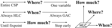
In this paper, we present PREPEAK+ as a reactive strategy that operates on the two dimensions 'when' and 'how much.' In particular, (a) we introduce a triggering strategy, PREPEAK, that tracks search performance and triggers HLC when search starts thrashing (i.e., when), and (b) choose to enforce HLC on a fraction of the (ordered) propagation queue and within a bounded time duration (i.e., how much).
We validate PREPEAK+ using as HLC the consistency property Partition-One Arc-Consistency (POAC) [Bennaceur and Affane, 2001; Balafrej et al., 2014]. This choice is justified by the fact that POAC is implemented with singleton tests and only standard GAC propagators (e.g., propagators of table constraints or global constraints), which probably makes it the easiest and most immediate HLC to implement in constraint solvers. We empirically show that PREPEAK+ (with POAC) outperforms GAC on all kinds of binary/non-binary and structured/unstructured CSPs. We re-iterate that PREPEAK+ is generic and can be used in combination with any HLC. Indeed, preliminary results on other consistencies are extremely encouraging.
The paper is structured as follows. Section 2 reviews background information. Section 3 reviews and organizes related work along the three identified dimensions. Section 4 describes our triggering strategy PREPEAK and Section 5 discusses our strategy of how much HLC to enforce. Section 6 evaluates our approach and Section 7 compares our approach to other techniques. Finally, Section 8 concludes this paper.
2 Background
A constraint network is defined by P = (X,D, C). X is a set of variables where a variable xi ∈ X has a finite domain dom(xi) ∈ D. A constraint ci ∈ C is given by its scope scope(ci) and its relation rel(ci): scope(ci) is the sequence of variables to which ci applies; rel(ci) is the set of combinations of |scope(ci)| values satisfying ci. A tuple belonging to rel(ci) ∩ ∏xi∈scope(ci) dom(xi) is called a support of ci. A solution of P assigns, to each variable, a value from its domain such that all the constraints are satisfied. The problem of deciding the existence of a solution is called a Constraint Satisfaction Problem (CSP) and is known to be NP-complete. To this day, backtrack search remains the only sound and complete algorithm for solving CSPs [Bitner and Reingold, 1975]. Search operates by assigning a value to a variable and backtracks when a dead-end is encountered.
After each variable assignment, constraint solvers enforce some consistency on the unassigned variables to remove values from their domains that are inconsistent, given the constraints with the current assignment and, thus, cannot participate in a solution [Haralick and Elliott, 1980; Sabin and Freuder, 1994]. Such filtering prunes 'barren' subtrees from the search space and can reduce thrashing and consequently the search effort. The higher the consistency level enforced during search, the stronger the pruning and the lesser the search effort. However, higher levels of consistency may take more time/space to enforce.
The most commonly enforced consistency property is Generalized Arc Consistency (GAC) [Mackworth, 1977]. A constraint network is GAC iff, for every constraint ci, and every variable x ∈ scope(ci), every value v ∈ dom(x) is consistent with ci (i.e., appears in some support of ci). Let (xi, vi) denote a variable-value pair, (xi, vi) ∈ P iff vi ∈ dom(xi). GAC(P ∪ {xi ← vi}) is the constraint network after assigning xi ← vi and running GAC. Singleton Arc-Consistency (SAC) ensures that for each (xi, vi) ∈ P, GAC(P ∪ {xi ← vi}) does not have any empty domain [Debruyne and Bessi`ere, 1997]. Testing GAC(P ∪ {xi ← vi}) is called a singleton test. A higher-level consistency property that has recently shown promise is Partition-One ArcConsistency (POAC) [Bennaceur and Affane, 2001]. A constraint network P = (X , D, C) is POAC iff P is SAC and for all (xi, vi) ∈ P, for all xj ∈ X, there exists vj ∈ dom(xj) such that (xi, vi) ∈ GAC(P ∪{xj ← vj}). POAC is guaranteed to enforce a higher-level consistency than SAC and SAC than GAC [Bennaceur and Affane, 2001].
Balafrej et al. [2014] introduced two algorithms for enforcing POAC, namely, POAC-1 and its adaptive version APOAC. In POAC-1, all the CSP variables are singleton tested, and the process is repeated over all the variables until a fixpoint is reached. In APOAC, the process is interrupted as soon as a given number of variables are processed, which depends on input parameters but is updated during search. Our experiments compare GAC, APOAC, PREPEAK+ with POAC as an HLC.
3 RelatedWork
We organize the related work along the three axes shown in Figure 1 and combinations of these dimensions.
Where: The consistency level is chosen based on some property of the variables and/or constraints. One can exploit structural properties of the constraint network, such as the neighborhood of a variable or a constraint [Freuder and Elfe,
1996; Wallace, 2015; Woodward et al., 2011], or some configuration of constraints [Karakashian et al., 2010]. Freuder and Wallace [1991] enforce arc consistency on a subproblem within a given distance (i.e., where) from the instantiated variable. Balafrej et al. [2013] and Woodward et al. [2014] exploit the degree of support that constraints provide to variable-value pairs, which is a structural property.
When: The consistency selected depends on search performance. Borrett et al. [1996] switch between backtrack algorithms, level of consistency enforced, and ordering heuristics by a complex combination of domain sizes, number of variables, and backtrack levels. Epstein et al. [2005] consider several strengths of AC-based consistencies depending on the depth of the search tree. Balafrej et al. [2015] use a multiarmed bandit at each depth of search tree to select between MAC, maxRPC, or POAC.
How much: Propagation is terminated before reaching a fixpoint. Such approaches focus on the propagation queue of a consistency algorithm. They either order the propagation queue according to some heuristic [Wallace and Freuder, 1992] or interrupt the consistency algorithm when the pruning effect of propagation has subsided [Balafrej et al., 2014] or the allocated time has elapsed [E´en and Biere, 2005; Geschwender et al., 2016].
Where and when: Some authors propose heuristics to dynamically switch from GAC to a stronger property on a selection of constraints (i.e., where) based on the amount of activity of the constraints during search (i.e., when). For example, Stergiou [2008] switches between GAC and maxRPC for binary CSPs and Paparrizou and Stergiou [2012] between GAC and maxRPWC for nonbinary CSPs.
Where and how much: Paparrizou and Stergiou [2017] propose a strategy for interrupting enforcing NeighborhoodSAC based on the amount of filtering it yields. For each singleton test on the considered variable, the filtering is interrupted (i.e., how much) unless the domain of any neighboring variable (i.e., where) becomes singleton.
4 When HLC: A Trigger-Based Strategy
We introduce our HLC-triggering strategy PREPEAK.
4.1 PREPEAK
The idea behind our reactive strategy is to monitor the 'progress' of search while maintaining some consistency property, such as GAC, in a d-way branching backtrack search. When search starts thrashing, we trigger some highlevel consistency (HLC), such as POAC, and keep enforcing it as long as it is beneficial. In order to determine that thrashing has reached a dangerous level, we propose to track the number of backtracks at each depth (or level) of the search tree. We advocate using the number of backtracks as a better indication of thrashing than the number of constraint checks (e.g., [Epstein et al., 2005]) or the number of nodes visited because the former depends on the number of constraints that apply to a variable and the latter depends on the variable's domain size. To this end, we store the number of times each level of the search tree was backtracked to in a vector btcounts[·] indexed by the corresponding level. The size of the vector is n + 1 where n is the number of variables in the problem. When an entry in this vector reaches some threshold value θ, we set peakd, identified as the 'peak' depth of thrashing, to the search depth corresponding to that entry. When search backtracks to a shallower depth than peakd, we enforce HLC as long as HLC is effective, then we revert to enforcing GAC after resetting to 0 all the counts in btcounts[·]. We call this approach PREPEAK because (a) it is based on identifying the peak depth to which search backtracks and (b) HLC is enforced up to this depth. Our goal is to 'hit hard' the future subproblem with HLC and reduce its size before the search reaches the peak depth again.
We present PREPEAK as simple modifications of the functions UNLABEL (Algorithm 1) and LABEL (Algorithm 2) of Prosser's 'classical' backtrack search algorithm [1993]. These modifications are obtained by adding the lines highlighted in the pseudocode. Below, we discuss only the lines corresponding to our modifications. Further, we declare btcounts[·] and peakd as global variables to the search procedure. We initialize all the entries of btcounts[·] to 0 and set peakd to 0 indicating that there is no active peak.
In Line 5 of UNLABEL (Algorithm 1), we increment the value of btcounts[h] where h is the depth to which we backtrack. If btcounts[h] reaches the threshold value θ, we set peakd to h to reduce the chance of thrashing at i (Line 6). We discuss the selection of the initial value of θ in Section 4.3.
It is in the function LABEL (Algorithm 2) that we must decide whether or not to enforce HLC. At every assignment of the current variable xi, we first enforce GAC (Line 6). At Line 7, if we find that a peak was identified (peakd > 0) and the current depth is shallower than the peak's depth (i ≤ peakd), we enforce HLC on the future subproblem recording the outcome of this call, for the given assignment, using the Boolean variables consistent and filtered (Line 8), where consistent indicates the consistency of the current path and filtered indicates whether or not HLC yielded any filtering. The Boolean variables HLCenforced and HLCfiltered indicate, for any tested assignment for the current variable, whether or not HLC was enforced (Line 9) and yielded filtering (Line 10), respectively. Note, once HLC is triggered, we
Algorithm 1: UNLABEL(i,consistent) unlabels variable xi Input: i: depth of failed variable; consistent: state of current path Output: depth of current variable 1 Restore domains of current and future variables 2 h ← i -1 3 dom(xh) ← dom(xh) \ {ASSIGNEDVALUE(xh)} 4 consistent ← dom(xh) ̸= ∅ 5 btcounts[h] ← btcounts[h] +1 6 if btcounts[h] = θ then peakd ← h 7 return hAlgorithm2: LABEL(i,consistent) instantiates variable xi Input: i: depth of current variable; consistent: state of current path Output: depth of current variable 1 consistent ← false 2 HLCenforced ← false 3 HLCfiltered ← false 4 foreach vi ∈ dom(xi) while not consistent do 5 xi ← vi 6 consistent ← GAC(P) 7 if consistent and peakd > 0 and i ≤ peakd then 8 (consistent , filtered ) ← HLC(P) 9 HLCenforced ← true 10 HLCfiltered ← HLCfiltered or filtered 11 if not consistent then dom(xi) ← dom(xi) \ {vi} 12 if HLCenforced then 13 if not consistent then θ ← rw · θ 14 else 15 ∀z btcounts [z] ← 0 16 peak d ← 0 17 if HLCfiltered then θ ← rf · θ 18 else θ ← rn · θ19 if consistent then return i +1 else return i
enforce it for all the tested values for the current variable xi.
We claim that, whenever we trigger HLC, it is timely to revise and update the triggering threshold, θ, given the recorded outcome of HLC. We distinguish three regimes:
- Wipeout: HLC effectively depletes the domain of xi by yielding a wipeout at every instantiation. It forces search to backtrack.
- Filtering: HLC yields some filtering, but finds a consistent assignment for xi and allows search to proceed to the next level.
- Neither: HLC does not yield any filtering at all (beyond what GAC may have filtered). Search proceeds to the next level with a consistent instantiation for xi.
We update the threshold value θ by multiplying its current value by a factor of rw (Line 13), rf (Line 17), or rn (Line 18), for each of the above regimes, respectively, as we argue below. We discuss these factors in Section 4.2.
The first regime (i.e., wipeout) 'reinforces' our belief in the usefulness of HLC and entices us to continue to enforce HLC as we backtrack by one or more levels. To this end, we do not reset the values of peakd or btcounts[·]. In the remaining two regimes, we are reserved about the usefulness of HLC and prevent it from triggering again too soon. Thus, we reset the values of both btcounts[·] and peakd (Lines 15 and 16). As a result, subsequent calls to the function LABEL do not enforce HLC until a new peak is detected.
4.2 Update Strategies for θ
The three identified regimes allow us to 'plug in' arbitrary strategies for updating θ, thus providing an opportunity to adjust PREPEAK's reactivity to the relative cost of the consistency properties enforced. We propose to use geometric laws similar to the one used for cutoff-value update in restarting randomized search [Walsh, 1999] θ ← r · θ with different values of the common ratio r for each of the regimes.
- Wipeout: We use rw = 1.2-1 (Line 13). 1
- Filtering: We use rf = 1.22 (Line 17).
- Neither: We use rn = 1.23 (Line 18).
The above strategies allow PREPEAK to adapt to the instance at hand by updating θ based on HLC's pruning effectiveness. Indeed, when it yields a domain wipeout (first regime), HLC is effectively reducing thrashing and its frequency is increased. Otherwise, the update strategies decrease HLC's triggering frequency more aggressively when HLC yields no filtering (third regime) than when it does (second regime).
4.3 Initializing the Threshold θ
Our reactive strategy enforces GAC until search starts thrashing, triggering HLC when backtracking 'reaches' the value of the threshold θ. If we choose too small an initial value for θ, HLC may trigger while GAC is still effective, which adds to the CPU cost. 2 If we choose too large a value, GAC may have run for too long in a barren subtree.
In PREPEAK, the distribution of the backtracks in the vector btcounts[·] varies depending on the problem instance, making the choice of the initial value of θ not straightforward. We investigated an alternative reactive strategy that triggers HLC based on the value of ∑nl=1 btcounts[l]. This study inspired the following initialization of θ for PREPEAK: we set θ to be the maximum value of btcounts[·] when ∑nl=1 btcounts[l] = n2 , thus, setting θ ← maxnl=1 (btcounts[l]). In other words, we identify the first peak and its depth by taking a snapshot of the backtrack profile after search executes n2 backtracks. We tested different values, such as various powers of n, various factors of n, the sum of domain sizes, and the ratio of the CPU times for enforcing GAC and HLC computed in a pre-processing step. We empirically found that values that are quadratic in the number of variables (e.g., n2 and sum of domain sizes) perform best, thus, we select n2 .
5 HowMuch HLC: Monitoring Propagation
We propose two mechanisms to control the early termination of HLC, namely, the size of the propagation queue and the time bound for running HLC. First, while ordering the elements of the propagation queue of the HLC algorithm based on the activity of a variable or constraint (e.g., dom/wdeg [Boussemart et al., 2004]), we allow only a fraction of the propagation queue to be processed. Second, we impose a bound on the duration of any call to HLC.
1 The value of 1.2 is a commonly used factor (e.g., [Walsh, 1999]) and provides a 'gentle' evolution. Other values tested (e.g., 1.1, 1.4, and 1.6) yielded qualitatively similar results.
2 We empirically noticed that the three update rules (Section 4.2) allow us to recover from starting with smaller values by dynamically adjusting the value of θ to the instance at hand, thus providing some robustness to our approach.
Let q be the number of elements in the propagation queue each time we trigger HLC. We terminate HLC as soon as either of the following two criteria is met:
- q2 elements of the propagation queue are processed or
- HLC has consumed a total CPU time q2 · TIME(GAC) where TIME(GAC) is the time spent on the last call to GAC prior to HLC (Line 6 of Algorithm 2).
Our approach is inspired from Balafrej et al. [2014], who noticed that POAC is too costly to be used on its own. They advocated to (a) order the variables in the propagation queue by the dom/wdeg ordering heuristic and (b) terminate POAC when the amount of filtering by POAC significantly drops. They proposed an adaptive strategy APOAC, based on a "10% learning, 90% exploitation"-learning strategy, which assumes that POAC is enforced at every step during search. PREPEAK cannot accommodate such a learning process because HLC is enforced only reactively.
Other mechanisms to monitor propagation may exist. For example, we can watch propagation during a given window of the propagation queue while sliding this observation window as long as filtering is 'active.' Alternatively, we can consider a sliding window of time. We tested combinations of such criteria. While the results were positive in general, they were unstable across benchmarks. As a lesson, we conclude that a fixed amount for each mechanism (i.e., queue and time) is simpler to implement, more stable, and as effective.
6 Experiments
We denote PREPEAK+ the combination of our when strategy (PREPEAK, Section 4) and our how-much strategy (Section 5). To validate our approach, we consider the problem of finding a single solution to a CSP using d-way branching backtrack search. We set up our experiments as follows. We choose POAC for the higher-consistency property and enforce it using the POAC-1 algorithm [Balafrej et al., 2014], where we exclude variables with singleton domains from the singleton tests.
We use the benchmark problems available from Lecoutre's website. 3 We test all available binary and non-binary CSPs, including Boolean, patterned, random, quasi-random, academic, and real-world benchmarks. We include all benchmarks with at least one instance with a primal graph of density less than 50%. Indeed, on high density networks, the impact of an instantiation on a future variable is immediately propagated by GAC while HLC typically yields no further filtering but costs predictable data-setup overhead. This selection results in a total of 138 benchmarks (57 non-binary and 81 binary) consisting of 4,077 instances (1,716 non-binary and 2,361 binary). The selected benchmarks have a mixture of instances with densities ≥ 50% and < 50%, however, only 137 instances of the 4,077 instances included have densities ≥ 50%. We setup our reactive strategies to first compute the density of an instance. If the density is ≥ 50%, we enforce GAC. Otherwise, we execute the reactive strategy. Our results include this computation time. We use a time limit of 60 minutes per instance and 8GB of memory.
3 www.cril.univ-artois.fr/∼lecoutre/benchmarks.html
In our tables, we report the number of instances solved by a given algorithm (#solved), the number of nodes visited averaged over instances completed by all algorithms (avg. NV), and the total CPU time in seconds computed over instances completed by any of the compared algorithms (∑CPU). When an algorithm does not terminate within the time allocated, we add 3,600 seconds to the CPU time and indicate with a > sign that the time reported is a lower bound. For techniques that run POAC, we report the average number of calls to POAC after enforcing GAC (#CallsPOAC). A value is in boldface when it is the best value in a given row.
We first show that PREPEAK+ performs better than either of its components. Then, we compare PREPEAK+ against GAC and APOAC using two different dynamic variableordering heuristics: dom/deg [Bessi`ere and R´egin, 1996] and dom/wdeg [Boussemart et al., 2004]. Finally, we introduce a visualization of the search process to provide a graphical interpretation of the good performance of our approach.
6.1 Putting Together 'When' and 'HowMuch'
In this experiment, we use the dom/wdeg variable-ordering heuristic. Table 1 shows the contributions of the two aspects 'when' (PREPEAK, Section 4) and 'how much' (interrupting propagation, Section 5) to the good performance of PREPEAK+. PREPEAK+ solves more instances than either
| Algorithm | PREPEAK+ | When | HowMuch |
|---|---|---|---|
| #Instances: 4,077 total; 2,131 | by all; 2,298 | by at least one | |
| #solved | 2,286 | 2,239 | 2,171 |
| ∑CPU [sec] | >356,778.1 | >610,958.6 | >915,738.6 |
| avg. NV | 568,072.7 | 123,224.9 | 10,925.7 |
| #CallsPOAC | 2,477.5 | 1,128.1 | 5,019.4 |
component taken individually, which shows the importance of combining the two orthogonal dimensions. The number of calls to POAC in PREPEAK+ is mostly controlled by the triggering strategy (i.e., 'when'), which by itself is more expensive than PREPEAK+ because POAC runs until a fixpoint. The right-most column enforces POAC with early termination (Section 5) at every node, yielding the smallest number of nodes visited but the largest CPU time. 'When' and 'how much' complete difference instances: only 2,131 instances are completed by both. Combining 'when' and 'how much' in PREPEAK+ allows it to solve instances not solved by both.
6.2 PREPEAK+ Versus GAC and APOAC
Table 2 compares the performance of GAC, APOAC, and PREPEAK+ under the dom/deg ordering heuristic. 4 PREPEAK+ solves the most instances and is the fastest algorithm.
4 Although dom/wdeg is generally more effective than dom/deg, the decisions made by dom/wdeg are considered too unstable to objectively allow comparing algorithms' performance. Researchers studying the performance of HLC during search typically use dom/deg in their experiments [Balafrej et al., 2015; Paparrizou and Stergiou, 2016; 2017].
| Algorithm | GAC | APOAC | PREPEAK+ |
|---|---|---|---|
| #Instances: 4,077 total; 1,891 by all; 2,205 by at least one | |||
| #solved | 2,036 | 2,058 | 2,173 |
| ∑CPU [sec] | >1,044,380.1 | >1,042,622.9 | >455,189.2 |
| avg. NV | 1,138,447.6 | 90,047.4 | 324,020.2 |
| #CallsPOAC | - | 30,911.5 | 686.1 |
Predictably, in terms of average nodes visited, APOAC explores the fewest and PREPEAK+ is closer to APOAC than to GAC despite the relatively few calls to POAC (686.1). We conclude that PREPEAK+ triggers HLC at the right place and in the right amount, thus validating our approach.
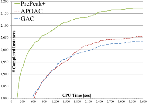
Figure 2 shows the cumulative number of instances completed by GAC, APOAC, and PREPEAK+ (on dom/deg) as time increases. Comparing GAC and APOAC, we see that GAC dominates APOAC on instances solved within 1,600 seconds, while APOAC dominates GAC after this point. This behavior motivates the need for HLC on difficult instances and illustrates its overhead on easier instances. By selectively triggering HLC, our strategy, PREPEAK+, dominates both GAC and APOAC.
Table 3 repeats the same experiment under dom/wdeg. The results are similar to those in Table 2: PREPEAK+ outperforms GAC and APOAC in terms of both number of instances solved and CPU time. Note that it would be incorrect to conclude that the CPU time of APOAC deteriorates from Table 2 to Table 3 because this measurement accounts for the number of instances completed in each experiment, which is different (i.e., 2,205 in Table 2 and 2,298 in Table 3).
| Algorithm | GAC | APOAC | PREPEAK+ |
|---|---|---|---|
| #Instances: 4,077 | total; 2,122 | by all; 2,298 | by at least one |
| #solved | 2,279 | 2,138 | 2,286 |
| ∑CPU [sec] | >372,433.4 | >1,095,125.8 | >356,778.1 |
| avg. NV | 480,897.9 | 23,472.9 | 319,453.4 |
| #CallsPOAC | - | 9,924.4 | 288.6 |
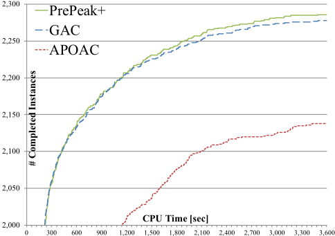
Figure 3 shows the cumulative number of instances completed by GAC, APOAC, and PREPEAK+ (on dom/wdeg) as CPU time increases. APOAC is clearly dominated by both GAC and PREPEAK+. For instances easily solved by GAC (i.e., solved in less than 300 seconds), PREPEAK+ has few calls to POAC because GAC is not thrashing. For the remaining harder instances, PREPEAK+ dominates GAC. PREPEAK+ remains competitive under dom/wdeg, which is known to dwarf the benefits of HLC.
Table 4 provides a finer examination of the results with dom/wdeg for a range of representative benchmarks, showing the number of instances in each benchmark in parentheses.
Rows 1-3 show benchmarks where PREPEAK+ significantly outperforms all others both in CPU time and the number of solved instances. For all remaining benchmarks, PREPEAK+ solves as many instances as the best algorithm.
APOAC solves more instances than GAC in rows 4 and 5, showing that HLC is required for these benchmarks. PREPEAK+ solves the same number of instances as APOAC, in faster CPU time, by selectively enforcing HLC. These benchmarks confirm the ability of our approach to mimic APOAC's performance when APOAC is needed.
In row 6 (QCP-15), GAC and APOAC are roughly equivalent, yet PREPEAK+ outperforms both in CPU time. For rows 7 and 8, GAC solves more instances than APOAC, however, PREPEAK+'s few calls to POAC allow it to slightly improve on the CPU performance of GAC. For rows 9-11, GAC significantly outperforms APOAC both in instance completions and CPU time: HLC is too costly on these benchmarks. However, PREPEAK+ is able to adapt to the situation with a CPU time similar to GAC's.
6.3 Visualizing Search Performance
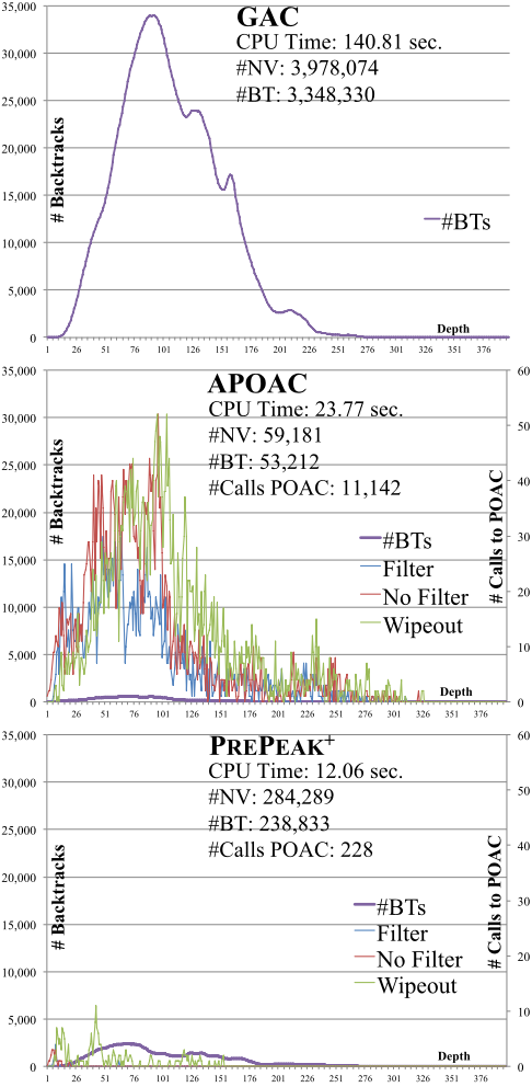
For a deeper insight into the behavior of search, we visualize the search execution, using dom/wdeg, on a CSP instance as shown in Figure 4, which 'profiles' search with GAC, APOAC, and PREPEAK+. In each of the three plots, we report, on the horizontal axis, the depth of the search tree. We plot the number of backtracks at each depth, accumulated throughout search (purple line), with the scale reported on the vertical axis to the left. We superimpose the cumulative number of calls to POAC (#Calls POAC) at each depth, with the scale reported on the vertical axis to the right. We split the number of calls to POAC into three cases: POAC yields wipeout (green line), POAC yields some filtering (blue line), and POAC yields no filtering at all (red line).
| Benchmark | GAC | APOAC | PREPEAK+ | |
|---|---|---|---|---|
| QCP-20 | # solved ∑CPU | 4 | 4 | 5 |
| 1 (15) | # solved | >5,328.7 | >4,861.0 | 2,762.9 |
| nengfa | 4 | 4 | 5 | |
| 2 (10) | ∑CPU | >3,820.6 | >4,235.9 | 2,321.0 |
| frb45-21 (10) | # solved ∑CPU | 7 | 0 >28,800.0 | 8 |
| 3 | # solved ∑CPU | >17,642.0 | 17 3,550.0 | 16,239.8 |
| 4 k-insertion (32) pseudo-ii | 16 >3,955.2 | 17 2,903.5 | ||
| 5 (41) | # solved ∑CPU | 9 >18,619.8 | 14 2,481.9 | 14 2,088.4 |
| QCP-15 | # solved | 15 | 15 | 15 |
| 6 (15) | ∑CPU | 1,310.0 | 1,248.4 | 1,213.5 |
| sgb-queen (50) | # solved ∑CPU | 14 | 12 | 14 5,692.0 |
| 7 | 5,712.9 | >9,969.6 | ||
| super-os | # solved | 9 | 1 | 9 |
| taillard5 (30) | ∑CPU | 11,971.1 | 11,969.8 | |
| super-os | 28 | 28 | ||
| 8 | >28,924.3 | |||
| 9 taillard-4 (30) | # solved ∑CPU | 7,647.2 | 22 >33,042.7 | 7,675.5 |
| geom | # solved | 100 | 98 | 100 |
| 10 (100) | ∑CPU | 7,254.3 | >28,365.6 | 7,372.8 |
| TSP-20 | # solved | 15 | 15 | 15 |
| (15) | ∑CPU | 276.5 | 298.6 | |
| 11 | 1,426.9 |
The backtrack curve (purple) shows that APOAC (middle) dramatically reduces the peak value reached by GAC (top) thanks to the large number of calls to POAC. Unfortunately, many of these calls are totally wasted (red curve) or likely of little impact (blue curve): In the middle plot, they compete with the wipeout calls (green curve). PREPEAK+ (bottom) makes significantly fewer calls to POAC and those calls are mostly effective (many more calls in green than in blue or red), which establishes that HLC is wisely exploited.
7 Comparison to Other Techniques
We identify two general strategies similar to PREPEAK+ in the sense that they are not designed for a particular HLC:
- In SAT solving, Wotzlaw et al. [2013] advocate reserving 10% of the CPU time for 'inprocessing' versus search. As a result, the more time is spent on search, the more 'inprocessing' is allowed.
- Balafrej et al. [2015] useMulti-Armed Bandits (MABs) at each search level to choose among a set of consistency algorithms.
We compare both techniques to PREPEAK+. 5 To level the playing field, we enhanced them both with our propagationmonitoring strategy (i.e., 'how-much HLC,' Section 5).
In our experiments on dom/wdeg (see Table 3), the fixed-ratio inprocessing approach solves 2,264 instances in
5 For the fixed-ratio inprocessing approach, we use POAC as HLC for 10% of the CPU time. For the MAB approach, we choose between GAC and POAC although the original paper also uses maxRPC, but it operates on only binary CSPs.
>413,634.6 seconds. It outperforms APOAC but performs worse than GAC. This strategy yields poor results because it is agnostic to 'where,' in the search space, an HLC is needed. Further, it is unable to react to the effectiveness of HLC (i.e., amount of pruning obtained by the HLC).
In our experiments on dom/wdeg (see Table 3), the MAB approach solves 2,253 instances in >529,767.9 seconds. It outperforms APOAC but performs worse than GAC. Because each MAB operates at a fixed level in search, using dom/wdeg adversarially affects the effectiveness and stability of a bandit's learning. Further, the MAB approach assesses the performance of a consistency call by the CPU cost of searching the subtree rooted at the call (regardless of which consistencies are used in the subtree). PREPEAK+ largely outperforms the MAB-based strategy for both dom/deg and dom/wdeg because PREPEAK+ uses the number of backtracks to assess search progress, which is a more precise measure of the HLC's effectiveness.
8 Conclusions
We introduce a simple, reactive, trigger-based strategy for advantageously enforcing a higher-level consistency during search and empirically validate our approach. Our experiments use POAC because it is perhaps the HLC that is the most readily portable to constraint solvers. However, preliminary results on other consistencies are extremely encouraging. The proposed visualization is an asset for in-vivo and post-mortem analysis and provides insight into the performance of search.
Acknowledgments
This research is supported by NSF Grant No. RI-111795 and RI-1619344. Robert Woodward was supported by an NSF GRF Grant No. 1041000 and a Chateaubriand Fellowship. This work was completed utilizing the Holland Computing Center of the University of Nebraska, which receives support from the Nebraska Research Initiative. Christian Bessiere was partially supported by the ANR projects Demograph (ANR-16-CE40-0028) and Contredo (ANR-16-CE33-0024).
@inproceedings{ijcai2018p193,
  title     = {A Reactive Strategy for High-Level Consistency During Search},
  author    = {Woodward, Robert J. and Choueiry, Berthe Y. and Bessiere, Christian},
  booktitle = {Proceedings of the Twenty-Seventh International Joint Conference on
               Artificial Intelligence, {IJCAI-18}},
  publisher = {International Joint Conferences on Artificial Intelligence Organization},
  editor    = {Jérôme Lang},
  pages     = {1390--1397},
  year      = {2018},
  month     = {7},
  note      = {Main track},
  doi       = {10.24963/ijcai.2018/193},
  url       = {https://doi.org/10.24963/ijcai.2018/193},
}
TY - CPAPER TI - A Reactive Strategy for High-Level Consistency During Search AU - Woodward, Robert J. AU - Choueiry, Berthe Y. AU - Bessiere, Christian T2 - Proceedings of the Twenty-Seventh International Joint Conference on Artificial Intelligence, IJCAI-18 PB - International Joint Conferences on Artificial Intelligence Organization PY - 2018 SP - 1390 EP - 1397 DO - 10.24963/ijcai.2018/193 UR - https://doi.org/10.24963/ijcai.2018/193 ER -Copied
Machine-readable versions of this paper, for tools and AI agents:





