
Compact-MDD: Efficiently Filtering (s)MDD Constraints with Reversible Sparse Bit-sets
Proceedings of the Twenty-Seventh International Joint Conference on Artificial Intelligence. Main track. Pages 1383-1389.
https://doi.org/10.24963/ijcai.2018/192
Keywords
- Constraints and SAT: Global Constraints
- Constraints and SAT: Constraint Satisfaction
- Constraints and SAT: Modeling;Formulation
Abstract
Multi-Valued Decision Diagrams (MDDs) are instrumental in modeling combinatorial problems with Constraint Programming.In this paper, we propose a related data structure called sMDD (semi-MDD) where the central layer of the diagrams is non-deterministic.We show that it is easy and efficient to transform any table (set of tuples) into an sMDD.We also introduce a new filtering algorithm, called Compact-MDD, which is based on bitwise operations, and can be applied to both MDDs and sMDDs.Our experimental results show the practical interest of our approach, both in terms of compression and filtering speed.
- [Amilhastre et al., 2014] Jerome Amilhastre, Helene Fargier, Alexandre Niveau, and Cédric Pralet. Compiling CSPs: A complexity map of (non-deterministic) multival- ued decision diagrams. International Journal on Artificial Intelligence Tools, 23(04), 2014.
- [Andersen et al., 2007] Henrik Andersen, Tarik Hadzic, John Hooker, and Peter Tiedemann. A constraint store based on multivalued decision diagrams. In Proceedings of CP'07, pages 118-132, 2007.
- [Bergman et al., 2014] David Bergman, André Ciré, and Willem van Hoeve. MDD propagation for sequence constraints. Journal of Artificial Intelligence Research, 50:697-722, 2014.
- [Bergman et al., 2016] David Bergman, André Ciré, Willem van Hoeve, and John Hooker. Decision diagrams for opti- mization. Springer, 2016.
- [Boussemart et al., 2016] Frédéric Boussemart, Christophe Lecoutre, and Cédric Piette. XCSP3: An integrated for- mat for benchmarking combinatorial constrained prob- lems. Technical Report arXiv:1611.03398, CoRR, 2016. Available from http://www.xcsp.org. Link
- [Bryant, 1986] Randal Bryant. Graph-based algorithms for Boolean function manipulation. IEEE Transactions on Computers, 35(8):677-691, 1986.
- [Cheng and Yap, 2008] Kenil Cheng and Roland Yap. Main- taining generalized arc consistency on ad-hoc r-ary con- straints. In Proceedings of CP'08, pages 509-523, 2008.
- [Cheng and Yap, 2010] Kenil Cheng and Roland Yap. An MDD-based generalized arc consistency algorithm for positive and negative table constraints and some global constraints. Constraints, 15(2):265-304, 2010.
- [Demeulenaere et al., 2016] Jordan Demeulenaere, Renaud Hartert, Christophe Lecoutre, Guillaume Perez, Laurent Perron, Jean-Charles Régin, and Pierre Schaus. Compact- Table: efficiently filtering table constraints with reversible sparse bit-sets. In Proceedings of CP'16, pages 207-223, 2016.
- [Dolan and Moré, 2002] Elizabeth Dolan and Jorge Moré. Benchmarking optimization software with performance profiles. Mathematical programming, 91(2), 2002.
- [Gange et al., 2011] Graeme Gange, Peter Stuckey, and Ra- doslaw Szymanek. MDD propagators with explanation. Constraints, 16(4):407-429, 2011.
- [Gent et al., 2007] Ian Gent, Chris Jefferson, Ian Miguel, and Peter Nightingale. Data structures for generalised arc consistency for extensional constraints. In Proceedings of AAAI'07, pages 191-197, 2007.
- [Hadzic et al., 2008] Tarik Hadzic, John Hooker, Barry O'Sullivan, and Peter Tiedemann. Approximate compi- lation of constraints into multivalued decision diagrams. In Proceedings of CP'08, pages 448-462, 2008.
- [Hoda et al., 2010] Samid Hoda, Willem van Hoeve, and John Hooker. A systematic approach to MDD-Based con- straint programming. In Proceedings of CP'10, pages 266-280, 2010.
- [Lecoutre, 2011] Christophe Lecoutre. STR2: Optimized simple tabular reduction for table constraints. Constraints, 16(4):341-371, 2011.
- [Perez and Régin, 2014] Guillaume Perez and Jean-Charles Régin. Improving GAC-4 for Table and MDD constraints. In Proceedings of CP'14, pages 606-621, 2014.
- [Perez and Régin, 2015] Guillaume Perez and Jean-Charles Régin. Efficient operations on MDDs for building con- straint programming models. In Proceedings of IJCAI'15, pages 374-380, 2015. IJCAI
- [Perez and Régin, 2017] Guillaume Perez and Jean-Charles Régin. Soft and cost MDD propagators. In Proceedings of AAAI'17, pages 3922-3928, 2017.
- [Perez, 2017] Guillaume Perez. Decision diagrams: con- straints and algorithms. PhD thesis, Université de Nice, 2017.
- [Rossi et al., 2006] Francesca Rossi, Peter van Beek, and Toby Walsh, editors. Handbook of Constraint Program- ming. Elsevier, 2006.
- [Verhaeghe et al., 2017] Hélène Verhaeghe, Christophe Lecoutre, Yves Deville, and Pierre Schaus. Extending compact-table to basic smart tables. In Proceedings of CP'17, pages 297-307, 2017.
- [Wang et al., 2016] Ruiwei Wang, Wei Xia, Roland Yap, and Zhanshan Li. Optimizing Simple Tabular Reduction with a bitwise representation. In Proceedings of IJCAI'16, pages 787-795, 2016. IJCAI
References were extracted automatically from the PDF and may contain errors.
Full text extracted automatically from the PDF; figures, tables and equations may differ. The PDF is the version of record.
1 Introduction
Constraint Programming (CP) is a general and flexible framework for modeling and solving combinatorial constrained problems [Rossi et al., 2006]. Many kind of constraints have been introduced in the literature, but general forms that are based on data structures such as tables, automatas, and MDDs (Multi-valued Decision Diagrams) remain quite popular. For example, over the past decade, many filtering algorithms have been proposed for table and MDD constraints, respectively leading to the state-of-the-art algorithms called Compact-Table [Demeulenaere et al., 2016] and MDD4R [Perez and R´egin, 2014]. In this paper, we focus our interest on decision diagrams [Bryant, 1986] for constraint reasoning, which is a hot topic; see, e.g., [Andersen et al., 2007; Hadzic et al., 2008; Hoda et al., 2010; Gange et al., 2011; Bergman et al., 2014; Amilhastre et al., 2014; Bergman et al., 2016; Perez and R´egin, 2017; Perez, 2017].
In theory, when dealing with finite domain variables, it is always possible to express a constraint c under the form of a table, which simply enumerates the tuples allowed by c, or an MDD whose paths indicate them. Clearly, tables and MDDs have the same expressive power, but the main advantage of MDDs is their ability to compress the set of tuples, possibly with an exponential space-saving. Hence, when compression is high, it is very relevant to convert tables intoMDDs, by using a procedure that identifies similar prefixes and suffixes of tuples. Unfortunately, it is known that different orderings on the variables (columns of the table) can lead to very different MDDs in term of size, and discovering the optimal order is an NP-hard task.
In this paper, we are interested in using decision diagrams for representing tables (while assuming an arbitrary ordering on the variables). We propose to relax one strong property of MDDs (out-determinism, which is the requirement that two arcs going out from the same node must be labeled differently). In this respect, we propose to refine the compression procedure by targeting a diagram that is no more an MDD. More precisely, the diagram generated by our procedure is an MVD (Multi-valued Variable Diagram) [Amilhastre et al., 2014], and because it admits a particular structure, basically representing two connected MDDs of approximately the same size (height), we shall call this structure an sMDD (semi-MDD).
Our contributions are summarized as follows: (i) a new structure called sMDD, adapted to the filtering of constraints, (ii) a new algorithm for converting any table into an sMDD, (iii) a new filtering algorithm enforcing Generalized Arc Consistency on constraints defined by sMDDs, and also MDDs, by relying on bit-set operations, as in [Wang et al., 2016; Demeulenaere et al., 2016], (iv) some experimental results showing that the number of nodes in sMDDs is usually far smaller than in equivalent MDDs, while leading to a faster filtering process compared to previous MDD approaches [Cheng and Yap, 2010; Perez and R´egin, 2014]. Results also show reduction of the time gap with Compact-Table.
2 Technical Background
A constraint network is composed of a set of variables and a set of constraints. Each variable x has an associated (finite) domain dom(x) containing the values that can be assigned to it; this current domain is included in the initial domain dom0 (x). Each constraint c involves an ordered set of variables, called the scope of c and denoted by scp(c), and is semantically defined by a relation rel(c) containing the tuples allowed for the variables involved in c. The arity of a constraint c is |scp(c)|. When the domain of a variable x is (becomes) singleton, we say that x is bound.
Given a sequence 〈x1, . . . , xr〉 of r variables, an r-tuple τ on this sequence of variables is a sequence of values 〈a1, . . . , ar〉, where the individual value ai is also denoted by τ[xi]. An r-tuple τ is valid on an r-ary constraint c iff ∀x ∈ scp(c), τ[x] ∈ dom(x), and τ is allowed by c iff
τ ∈ rel(c). A support on c is a tuple that is both valid on c and allowed by c. A literal is a pair (x, a) where x is a variable and a a value. A literal (x, a) is Generalized ArcConsistent (GAC) on c iff there is a support τ on c such that τ[x] = a. A constraint c is GAC iff any literal (x, a) such that x ∈ scp(c) and a ∈ dom(x) is GAC on c.
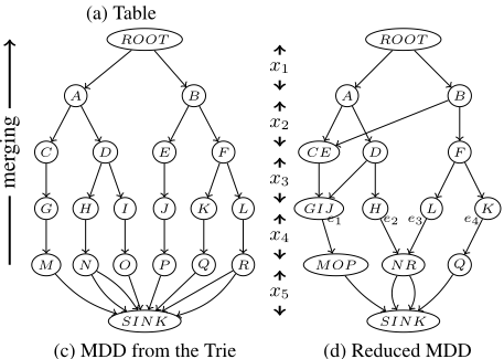
A directed graph is composed of nodes and arcs. Each arc has an orientation from one node, the tail of the arc, to another node, the head of the arc. For a given node ν, the set of arcs with ν as tail (resp., head) is called the set of outgoing (resp., incoming) arcs of ν. A (arc-)labeled directed graph is a directed graph such that a label is associated with each arc. A node is in-d (in-deterministic) iff no two incoming arcs have the same label, in-nd otherwise. A node is outd (out-deterministic) iff no two outgoing arcs have the same label, out-nd otherwise. A directed acyclic graph (DAG) is a (finite) directed graph with no directed cycles. An MVD (Multi-valued Variable Diagrams) [Amilhastre et al., 2014], associated with a constraint of arity r, is a layered DAG, with one special root node at level 0, denoted by ROOT, r layers of arcs, one layer for each variable of the constraint scope 〈x1, . . . , xr〉, and one special sink node at level r, denoted by SINK. The arcs going from level i - 1 to level i are on the variable xi: any such arc is labeled by a value in dom0 (xi). A valid path in an MVD is a path from the root to the sink such that the label of each involved arc going from level i-1 to i is a value in dom(xi). The set of supports of a constraint c defined by an MVD M corresponds to the valid paths in M. One classical type of MVD is the Multi-valued Decision Diagram (MDD) [Bryant, 1986], which guarantees that each node is out-d (each node at level i has at most |dom0 (xi)| outgoing arcs, labeled with different values), but possibly innd. An example is given in Fig. 1d. We now introduce the data structure studied in this paper.
Definition 1 A semi-MDD, or sMDD, is an MVD such that each node at a level < ⌊ r2 ⌋ is out-d and each node at a level > ⌊ r2 ⌋ +1 is in-d.
This means that in an sMDD, a node at a level < ⌊ r2 ⌋ is possibly in-nd, and a node at a level > ⌊ r2 ⌋ + 1 is possibly out-nd. Also, a node at level ⌊ r2 ⌋ or ⌊ r2 ⌋+1 is possibly both in-nd and out-nd. Level ⌊ r2 ⌋ is chosen to minimize the upper-bound of the number of nodes. An example is given in Fig. 2h.
A table constraint c is such that rel(c) is explicitly defined by listing the tuples that are allowed by c. A MVD (resp., MDD and sMDD) constraint c is such that rel(c) is defined by a MVD (resp., MDD and sMDD).
3 FromTables to Diagrams
The table of an extensional constraint c can be compactly represented by a trie [Gent et al., 2007] in which successive levels are associated with successive variables in the scope of c. A trie can be further reduced by merging nodes 1 , so as to obtain an MDD.
3.1 Generating (Reduced) MDDs
Reduction algorithms for generating diagram decisions from tables (sets of tuples) have been proposed in the literature. A
1 In the spirit of the Hopcroft algorithm for DFA minimization.
| x1 | x2 | x3 | x4 | x5 |
|---|---|---|---|---|
| 0 | 0 | 0 | 0 | 1 |
| 0 | 1 | 0 | 1 | 0 |
| 0 | 1 | 0 | 1 | 1 |
| 0 | 1 | 1 | 0 | 1 |
| 1 | 0 | 0 | 0 | 1 |
| 1 | 1 | 0 | 0 | 0 |
| 1 | 1 | 1 | 0 | 0 |
| 1 | 1 | 1 | 0 | 1 |
| 0 | 0 | 0 | 0 | 1 |
| 1 | 0 | 1 | 01 | |
| 1 | 0 | 1 | ||
| 1 | 0 | 0 | 0 | 1 |
| 1 | 0 | 0 | 0 | |
| 1 | 0 | |||
| 01 |
Figure 1: Reducing a Table into an MDD
first algorithm based on a breadth-first bottom-up exploration, was proposed in [Bryant, 1986] for BDDs (Boolean Decision Diagrams), and a second algorithm, using a dictionary and called mddify, was proposed in [Cheng and Yap, 2010; 2008] for MDDs. More recently, pReduce [Perez and R´egin, 2015] has been shown to admit a better worst-case time complexity than mddify.
Fig. 1 illustrates the creation of an MDD in the spirit of pReduce. Initially, we consider a constraint c defined by the table shown in Fig. 1a. First, the trie corresponding to this table is created 2 , Fig. 1b, and a (non-reduced) MDD can be easily derived from this trie, Fig. 1c 3 . Then, the MDD is reduced by successively merging nodes when possible, from bottom to top. Merging is done by finding nodes having similar sets of outgoing arcs. Two sets of outgoing arcs are similar if they have the same cardinality, and for each arc in one set, there is an arc in the other set with the same label (value) and the same head. In our example, you can observe that nodes M, O and P have only one outgoing arc, each one labeled with 1 and reaching SINK. Hence, these nodes can be merged (node MOP in Fig. 1d). The MDD resulting from this iterative merging process is shown in Fig. 1d.
3.2 Generating sMDDs
Now, we propose to refine the reduction procedure by targeting a diagram that is an sMDD. The interest is that such structure is expected to contain less nodes (this issue is discussed later), and that efficient algorithms can be defined on sMDDs. The algorithm we propose is composed of five main steps, and is called sReduce. First, the initial table is split in two main parts:
2 Here, for simplicity a table structure is kept in Fig. 1b.
3 Dashed and plain edges stand for labels with values 0 and 1, respectively.
- the p-table (table for the prefixes) corresponding to a restriction of the table to its first ⌊ r2 ⌋ columns (or variables),
- the s-table (table for the suffixes) corresponding to a restriction of the table to its last r - ⌊ r2 ⌋ - 1 columns (or variables),
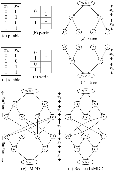
At this point, note that all variables, except one, are involved in one of these two partial tables. On our example with r = 5, we obtain a p-table with 2 columns (corresponding to x1 and x2) and an s-table with 2 columns (corresponding to x4 and x5). The missing column (for variable x3) will be considered in a later stage.
Second, duplicates are removed from the p-table (resp. s-table), which is then sorted using a lexicographic (resp. colexicographic 4 ) order. Considering again the initial table depicted in Fig. 1a, after these three steps, we obtain the ptable and the s-table shown in Fig. 2a and 2d.
Third, we build some equivalent tables sharing prefixes and suffixes (we call them p-trie and s-trie). Equivalent trees are naturally derived from them (we call them p-tree and s-tree). Importantly, the order of the columns is preserved, and we start with a special root node for the p-tree whereas we finish with a special sink node for the s-tree. An illustration is given by figures 2b, 2c, 2e and 2f.
Fourth, for each tuple τ in the initial table, an arc is built. It links the node in the p-tree corresponding to the end of the prefix of τ and the node in the s-tree corresponding to the start of the suffix of τ. This arc is labeled with the value for the intermediate variable, which was involved neither in the p-table nor in the s-table. We obtain a new diagram, depicted in Fig. 2g, where arcs have been added for x3.
Fifth, "classical" reduction is performed twice. On the one hand, from bottom to top, merging can be conducted by starting from the nodes that were leaves in the p-tree. For merging, the algorithm searches for similarities between sets of outgoing arcs. As an illustration, let us consider nodes C and E in Fig. 2g. These two nodes have both one outgoing arc with the same label 0 and the same head: therefore, they can be merged (node CE in Fig. 2h). On the other hand, from top to bottom, merging can be conducted by starting from the nodes that had no parent in the s-tree. For merging, the algorithm searches now for similarities between sets of incoming arcs. As an illustration, observe how nodes H and J in Fig. 2g can be merged (node HJ in Fig. 2h). The graph obtained after complete reduction is depicted in Fig. 2h.
Proposition 1 The graph obtained after executing sReduce on any specified table is an sMDD.
Proof: Before executing merging operations, the diagram (at the end of step 4) is an sMDD, by construction. Merging conducted in the first (bottom-up) pass preserves out-determinism of any node at a level < ⌊ r2 ⌋, while merging conducted in the second (top-down) pass preserves indeterminism of any node at a level > ⌊ r2 ⌋ + 1.
4 Ordering is done by reading numbers from right to left.
Note that the complexity of sReduce is basically the same as pReduce as operations are essentially the same (sorting and merging).
One interest of sMDDs over MDDs is the potential reduction of the number of nodes. Assuming an uniform variable domain size equal to d, the number of nodes in the initial trie is O(dr ) for the MDD while it is O(dr/2 ) for the sMDD. The gain can thus be very substantial although merging renders precise predictions difficult to make. On our example, from the same table, the generated MDD contains 14 nodes and 19 arcs, and the sMDD 12 nodes and 18 arcs.
4 Compact-MDD
In this section, we describe a new filtering algorithm that can be applied to any MVD (and so, to any MDD and sMDD). It is called Compact-MDD (or CMDD), and borrows some principles from CT [Demeulenaere et al., 2016] and MDD4R [Perez and R´egin, 2014]. Its description is given under the form of an object-oriented programming class in Algorithm 1.
4.1 Data Structures
As fields of Class Constraint-CMDD, we first find scp for representing the scope 〈x1, . . . , xr〉 of c and currArcs for representing the current set of valid arcs of the diagram. More precisely, a reversible sparse bit-set from Class RSparseBitSet, as described in [Demeulenaere et al., 2016], is associated with each variable x of scp: currArcs[x] keeps track of the valid arcs on x. Each arc in the diagram admits an associated bit in currArcs: the arc is valid iff the bit is set to 1. Note that this is similar to currTable that keeps track of the valid tuples in CT. As an example, for the MDD in Fig. 1d, currArcs[x2] and currArcs[x3] respectively correspond to sequences of 4 and 5 bits (all set to 1, initially). In this data structure, one field is words, an array of w-bit words (e.g., w = 64), which defines the current value of the bit-set. Each reversible sparse bit-set has another field: a bit-set called mask that is used to perform and record intermediate computations. Interestingly, operations on mask are optimized so as to only consider non-zero words (i.e., words with not all bits set to 0).
We now succinctly describe the methods in RSparseBitSet. Method isEmpty() simply checks whether the number of non-zero words is different from zero. Method clearMask() sets to zero all words of mask whereas Method reverseMask() reverses all words of mask. Method addToMask() applies a word by word logical bit-wise or operation. Finally, Method intersectIndex() checks if a given bit-set intersects with the current bit-set: it returns the index of the first word where the intersection is non-zero, -1 otherwise. For the sake of simplicity, we shall use currArcs[x][i] as a shortcut for currArcs[x].words[i], and currArcs[x].intxn as a shortcut for currArcs[x].intersectIndex.
We also have three fields S val , S sup and lastSizes in the spirit of STR2 [Lecoutre, 2011]. The set S val contains variables whose domains have been reduced since the previous call to CMDD on c. To set up S val , we need to record the domain size of each variable x right after the execution of CMDD on c: this value is recorded in lastSizes[x]. The set S sup contains unbound variables whose domains contain each at least one value for which a support must be found. These two sets allow us to restrict loops on variables to relevant ones. To ease computations, at each level we find three types of precomputed bit-sets: these bit-sets are never modified. First, supports[x, a] indicates for each arc on the variable x whether or not the value a is initially supported by this arc (bit set to 1 iff a is supported). Second, arcsT[ν, x] and arcsH[x, ν ′ ] indicates for each arc on x whether ν and ν ′ are respectively the tail and the head of this arc. Fig. 3 displays these structures associated with x4 in the MDD depicted in Fig. 1d. Finally, we have dynamic bit-sets for handling socalled residues. We shall see their role when describing the algorithm.
| e1 | e2 | e3 | e4 | |
|---|---|---|---|---|
| supports[x4, 0] supports[x4, 1] | 1 0 | 0 1 | 1 0 | 1 0 |
| arcsT[GIJ, x4] arcsT[H, x4] arcsT[L, x4] arcsT[K, x4] | 1 0 0 0 | 0 1 0 0 | 0 0 1 0 | 0 0 0 1 |
| arcsH[x4,MOP] arcsH[x4, NR] arcsH[x4, Q] | 1 0 0 | 0 1 0 | 0 1 0 | 0 0 1 |
4.2 Algorithm
The main method in Constraint-CMDD is enforceGAC(). After the initialization of the sets S val and S sup , calling updateGraph() allows us to update the graph, and more specifically currArcs to filter out (indices of) arcs that are no more valid. Once the graph is updated, it is possible to test whether each value has still a support, by calling filterDomains(). If ever a domain wipe-out (failure due to a domain becoming empty) occurs, an exception is thrown during the update of the graph (and so, this is not directly managed in this main method). At the end of enforceGAC(), lastSizes is updated in view of the next call.
Updating the Graph
As in MDD4R, the goal of updateGraph() is to remove the arcs that are no more part of a valid path. An arc can be:
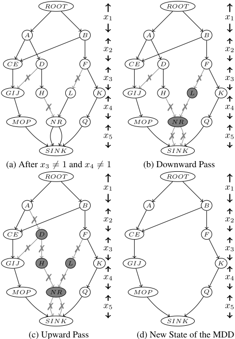
(i) trivially removed when the value of the label of the arc has been removed from the variable domain (since the previous call) (ii) or untrivially removed when all paths involving the arc are no more valid. Method updateGraph() follows this observation: it identifies first the arcs that can be trivially removed before identifying those that can be untrivially removed. Fig. 4 illustrates the whole updating process, considering the effect of having two deleted values on the MDD depicted in Fig. 1d. We shall refer to this illustration all along the description of this part of the algorithm.
In Method updateGraph(), after initializing all masks associated with the variables in the scope of the constraint, all arcs that can be trivially removed are handled by calling updateMasks(). For each variable x ∈ S val , i.e., each variable x whose domain has changed since the last time the filtering algorithm was called, updateMasks() operates on the associated masks. This method assumes an access to the set of values ∆x removed from dom(x) since the last call to enforceGAC(). There are two ways of updating the masks (before updating currArcs from these masks, later): either incrementally or from scratch after resetting as proposed in [Perez and R´egin, 2014]. This is the strategy implemented in updateMasks(), by considering a reset-based computation when the size of the domain is smaller than the number of deleted values. In case of an incremental update (line 16), the union of the arcs to be removed is collected by calling addToMask() for each bit-set (of supports) corresponding to removed values, whereas in case of a reset-based update (line 19), we perform the union of the arcs to be kept. To get masks ready to apply, we just need to reverse them when they have been built from present values. Unlike CT, the update of currArcs from the computed masks is not done immediately. Fig. 4a shows in gray the arcs that are added to the masks.
Last but not least, we need now to determine which arcs can be untrivially removed: this is achieved by calling the methods propagateDown() and propagateUp(), which, similarly to MDD4R, perform two passes on the diagram. During the downward (resp., upward) pass, each level is examined from the root (resp., sink) to the sink (resp., root) 5 .
In Method propagateDown(), for a specified variable xi, provided that some arcs on xi have been removed (the presence of arcs trivially removed are tested at Line 24 with xi ∈ S val , and the presence of arcs untrivially removed are given by the Boolean variable localChange), we have to process (and propagate) them. To start, currArcs is first updated (Line 25), and if no more arcs on xi remain, a backtrack is forced because there is necessarily a domain-wipe-out. If xi is not the last variable in the scope of the constraint, we have to deal with xi+1. Specifically, every node 6 ν that is the tail of a currently valid arc on xi+1 is tested: when there is no more valid arcs on xi with ν as head, all arcs on xi+1 with ν as tail are then untrivially removed. In other words, if there is no more valid incoming arc for a node ν at level i, then all outgoing arcs of ν become invalid: this is implemented by the
5 Actually, we can start propagation from the first and last unbound variables. For experiments, we used this code optimization.
6 Those are maintained in practice in a reversible sparse-set as in [Perez and R´egin, 2014].
Algorithm 1: Class Constraint-CMDD
1 Method enforceGAC() 2 S val ← {x ∈ scp : lastSizes[x] ̸= |dom(x)|} 3 S sup ← {x ∈ scp : |dom(x)| > 1} 4 updateGraph() 5 filterDomains() 6 foreach variable x ∈ S val ∪ S sup do 7 lastSizes[x] ← |dom(x)| 8 Method updateGraph() 9 foreach variable x ∈ scp do 10 currArcs[x].clearMask() 11 updateMasks() 12 propagateDown(x1, false) 13 propagateUp(xr, false) 14 Method updateMasks() 15 foreach variable x ∈ S val do 16 if |∆x| < |dom(x)| then // Incremental update 17 foreach value a ∈ ∆x do 18 currArcs[x].addToMask(supports[x, a]) 19 else // Reset-based update 20 foreach value a ∈ dom(x) do 21 currArcs[x].addToMask(supports[x, a]) 22 currArcs[x].reverseMask() 23 Method propagateDown(xi, localChange) 24 if xi ∈ S val or localChange then 25 currArcs[xi ].removeMask() 26 if currArcs[xi].isEmpty() then 27 throw Backtrack 28 if xi ̸= xr then 29 localChange ← false 30 foreach node ν ∈ {ν : currArcs[xi+1].intxn(arcsT[ν, xi+1]) ̸= -1} do 31 j ← residuesH[xi, ν] 32 if currArcs[xi][j] & arcsH[xi, ν][j] = 064 then 33 j ← currArcs[xi] .intxn(arcsH[xi, ν]) 34 if j ̸= -1 then 35 residuesH[xi, ν] ← j 36 else 37 currArcs[xi+1] .addToMask(arcsT[ν, xi+1]) 38 localChange ← true 39 propagateDown(xi+1, localChange) 40 else if xi ̸= xr then 41 propagateDown(xi+1, false) 42 Method propagateUp(xi, localChange) /* Similar to propagateDown with x1 instead of xr, xi-1 instead of xi+1, inverted use of arcsT and arcsH, inverted use of residuesT and residuesH. */ 43 Method filterDomains() 44 foreach variable x ∈ S sup do 45 foreach value a ∈ dom(x) do 46 i ← residues[x, a] 47 if currArcs[x][i] & supports[x, a][i] = 064 then 48 i ← currArcs[x].intxn(supports[x, a]) 49 if i ̸= -1 then 50 residues[x, a] ← i 51 else 52 dom(x) ← dom(x) \ {a}code at Lines 29..38. Note that the search of supporting arcs is improved by keeping track in residuesH of the last valid incoming arc, and starting with it. This increases the odds of not testing too many words of currArcs. Also, note how the variable localChange becomes true as soon as an arc is untrivially removed.
Fig. 4b shows the behavior of downward propagation on our example. For the two first levels, nothing happens. However, at the level of x3, we can see that all incoming arcs of the node L have been removed. Hence, the outgoing arcs of L are added to the mask associated with the next level, and removed when reaching this level. On the other hand, the node GIJ has still one valid incoming arc. Fig. 4c shows the result of upward propagation (after the downward one has been completed).
Filtering Domains
The process of filtering domains is very similar to that described in CT [Demeulenaere et al., 2016]. This is given by Method filterDomains() in Algorithm 1. For each remaining unbound variable x in S sup , and each value a in dom(x), the intersection between the valid arcs on x, currArcs[x], and the arcs labeled with value a, supports[x, a], determines if a is still supported. An empty intersection means that a can be deleted, at Line 52. This is correct because all "remaining" arcs in currArcs[x] are necessarily part of a valid path in the graph. The search of supports starts by using residues.
Back to our example, remaining arcs as defined by currArcs corresponds to the MDD depicted in Fig. 4d. Regarding x5, currArcs[x5] is 1001. Because supports[x5, 0] is 0101 and supports[x5, 1] is 1010, we can deduce (from bitwise intersections) that both values are still valid for x5.
One can show that CMDD enforces GAC (proof omitted, due to lack of space). Overall, the worst-case time complexity of CMDD is O(max(n, d)r aw ), where r is the arity, d the greatest domain size, n (a) the maximum number of nodes (arcs) per level, and w the size of the computer words. Indeed, updateMasks(), propagateDown()+propagateUp() and filterDomains() are respectively O(dr aw ), O(nr aw ) and O(dr aw ). It has to be compared with the worst-case time complexity of CT, which is O(dr tw ) with t being the size of the table.
Interestingly enough, the main features of diagrams generated by sReduce are substantially different from those generated by pReduce: the number of nodes can be dramatically lower while the number of arcs can be slightly higher (this will be confirmed by our experimental results). If we reasonably assume that d < n, the complexity of CMDD becomes O(rn aw ). Hence, what we can expect is that executing CMDD on sMDDs will be beneficial (because highly decreasing n has a stronger impact than slightly increasing a).
5 Experimental Results
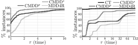
In our system, we have implemented pReduce, MDD4R [Perez and R´egin, 2014], CT [Demeulenaere et al., 2016], and the two algorithms proposed in this paper, namely, sReduce and CMDD. We have conducted an experimentation on the 4, 111 available XCSP3 instances [Boussemart et al., 2016] that only contain table constraints. We have compared the relative efficiency of MDD4R (after executing pReduce to convert tables), CMDDp (i.e., CMDD after executing pReduce), CMDDs (i.e., CMDD after executing sReduce) and CT (on the original tables). We have filtered out the instances taking less than 2 seconds or leading to a time out (10 minutes) for all algorithms. Results are reported using performance profiles [Dolan and Mor´e, 2002]. A performance profile is a cumulative distribution of the improved performance of an algorithm s ∈ S compared to other algorithms of S over a set I of instances: ρs(τ) = 1 |I| × |{i ∈ I : ri, s ≤ τ}| where the performance ratio is defined as ri, s = ti, s min{ti, s|s∈S} with ti, s the value of the mesured unit (here, number of nodes, number of edges or time) obtained with algorithm s ∈ S on instance i ∈ I. A ratio ri, s = 1 thus means that s is the best on instance i.
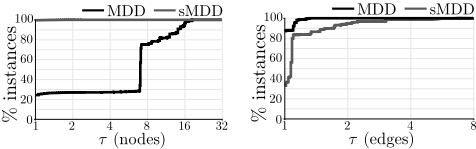
We first compared sReduce with pReduce. Similar execution times were observed for sReduce and pReduce. Concerning the size of the diagrams, Fig. 5 shows two performance profiles that allow us to compare globally the number of nodes and arcs in the generated MDDs and sMDDs for all the tables involved in our benchmark (around 230, 000 tables of arity greater than or equal to 3). As we predicted, the number of nodes is significantly reduced in the generated sMDDs (more than a factor 8 for at least 70% of the tables), while the number of arcs tends to be slightly higher.
On the left of Fig. 6, execution times of MDD4R, CMDDp and CMDDs are compared. Times are given for a complete exploration of the search space (i.e., to find all solutions), using each time the same variables and values choices. Clearly, CMDD outperforms MDD4R, even when it is executed on "simple" MDDs. Using sMDDs just makes it more robust. For example, CMDDs , CMDDp and MDD4R are at least 2 times slower than the best (virtual) algorithm on 5%, 20% and 35% of the instances, respectively. On the right of Fig. 6, CT is additionally considered. In general, CT still outperforms decision diagram approaches, but the gap is reduced: 40% of the instances are solved by CMDDs within a factor 2 compared to the time taken by CT, instead of 5% previously with MDD4R.
It is important to note that these global results do not tell the entire story. Indeed, when the compression is high, using decision diagrams remains the appropriate approach. For example, on the instance pigeonsPlus-11-06, the execution times of CT, MDD4R, CMDDp and CMDDs are respectively T.O.(> 600s), 328s, 128s and 126s. This confirms the real interest of approaches based on decision diagrams.
6 Conclusion
We have proposed an original variant of decision diagrams for representing (table) constraints, and have introduced an original efficient filtering algorithm, based on it. The new algorithm, CMDD, outperforms the state-of-the-art algorithm MDD4R, and is close to CT in general. Interestingly, when the compression is high, CMDD becomes the fastest approach. As future work, we would like to study if sMDDs could represent other constraints. We also plan, following the extension of CT to Basic Smart Table [Verhaeghe et al., 2017], to adapt the CMDD algorithm to handle Basic Smart MVD, i.e., MVD with edges labelled by a unary expressions.
Acknoledgements
The second author is supported by the project CPER Data from the "Hauts-de-France".
@inproceedings{ijcai2018p192,
  title     = {Compact-MDD: Efficiently Filtering (s)MDD Constraints with Reversible Sparse Bit-sets},
  author    = {Verhaeghe, Hélène and Lecoutre, Christophe and Schaus, Pierre},
  booktitle = {Proceedings of the Twenty-Seventh International Joint Conference on
               Artificial Intelligence, {IJCAI-18}},
  publisher = {International Joint Conferences on Artificial Intelligence Organization},
  editor    = {Jérôme Lang},
  pages     = {1383--1389},
  year      = {2018},
  month     = {7},
  note      = {Main track},
  doi       = {10.24963/ijcai.2018/192},
  url       = {https://doi.org/10.24963/ijcai.2018/192},
}
TY - CPAPER TI - Compact-MDD: Efficiently Filtering (s)MDD Constraints with Reversible Sparse Bit-sets AU - Verhaeghe, Hélène AU - Lecoutre, Christophe AU - Schaus, Pierre T2 - Proceedings of the Twenty-Seventh International Joint Conference on Artificial Intelligence, IJCAI-18 PB - International Joint Conferences on Artificial Intelligence Organization PY - 2018 SP - 1383 EP - 1389 DO - 10.24963/ijcai.2018/192 UR - https://doi.org/10.24963/ijcai.2018/192 ER -Copied
Machine-readable versions of this paper, for tools and AI agents:





