Simpler and Faster Algorithm for Checking the Dynamic Consistency of Conditional Simple Temporal Networks

1 Overview

A Conditional Simple Temporal Network (CSTN) is a data structure for reasoning about time in domains where some constraints may apply only in certain scenarios. For example, a patient who tests positive for a certain disease may need to receive care more urgently than someone who tests negative. Conditions in a CSTN are represented by propositional letters whose truth values are not controlled, but instead observed in real time. Just as doing a blood test generates a positive or negative result that is only learned in real time, the execution of an observation time-point in a CSTN generates a truth value for its corresponding propositional letter. An execution strategy for a CSTN specifies when the time-points will be executed. A strategy can be dynamic in that its decisions can react to information from past observations. A CSTN is said to be dynamically consistent (DC) if it admits a dynamic strategy that guarantees the satisfaction of all relevant constraints no matter which outcomes are observed during execution.

Different varieties of the DC property have been defined that differ in how reactive a dynamic strategy can be. Tsamardinos

Roberto Posenato

Department of Computer Science University of Verona, Italy roberto.posenato@univr.it

et al. [2003] stipulated that a strategy can react to an observation after any arbitrarily small delay. Comin et al. [2015] defined ϵ-DC, which assumes that a strategy's reaction times are bounded below by a fixed ϵ > 0. Finally, three different versions of DC for strategies that can react instantaneously (i.e., after zero delay) have been defined: IR-DC [Hunsberger et al., 2015]; 0-DC and π-DC [Cairo et al., 2016].

Several approaches to DC-checking algorithms have been presented to address the different flavors of DC [Tsamardinos et al., 2003; Cimatti et al., 2014; 2016; Comin and Rizzi, 2015], but the approach based on the propagation of labeled constraints [Hunsberger et al., 2015; Hunsberger and Posenato, 2016] is the only one that has been demonstrated to be practical. Three variations of their DC-checking algorithm have been presented: one for DC, one for ϵ-DC, and one for IR-DC. This paper focuses on their IR-DC-checking algorithm.

Subsequently, Cairo et al. [2016] showed that the 0-DC semantics (i.e., the ϵ-DC semantics where ϵ = 0) had a serious flaw: it allows a kind of circular dependence among simultaneous observations. To correct this, their π-DC semantics requires a strategy to specify an order-of-dependence among simultaneous observations. Whether the IR-DC semantics is similarly flawed and, if so, what the consequences would be for the IR-DC-checking algorithm, remained open questions.

This paper (1) shows that the IR-DC semantics is also flawed; (2) shows that one of the constraint-propagation rules from the IR-DC-checking algorithm is not sound with respect to the IR-DC semantics; (3) presents a simpler algorithm, called the π-DC-checking algorithm; (4) proves that the new algorithm is sound and complete with respect to the π-DC semantics; and (5) empirically evaluates the new algorithm.

2 Background

Dechter et al. [1991] introduced Simple Temporal Networks (STNs) to facilitate reasoning about time. An STN comprises real-valued variables, called time-points, and binary difference constraints on those variables. Typically, an STN includes a time-point, Z, whose value is fixed at zero. A consistent STN is one that has a solution as a constraint satisfaction problem.

Tsamardinos et al. [2003] presented CSTNs, which augment STNs to include observation time-points and their associated propositional letters. In a CSTN, the execution of an observation time-point P? generates a truth value for its associated letter p. In addition, each time-point can be labeled by a conjunction of literals specifying the scenarios in which that time-point must be executed. Later work generalized CSTNs to also include labels on constraints [Hunsberger et al., 2012].

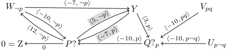
Fig. 1 shows a sample CSTN in its graphical form, where the nodes represent time-points, and the directed edges represent binary difference constraints. In the figure, Z is fixed at 0; and P? and Q? are observation time-points whose execution generates truth values for p and q, respectively. Q? being labeled by p indicates that Q? is executed only if p is observed to be true; and the edge from U to Q? being labeled by p¬q indicates that it applies only in scenarios where p is true and q is false. The dashed edges are generated by the IR-DCchecking algorithm [Hunsberger et al., 2015], discussed later.

Tsamardinos et al. [2003] noted that for any reasonable CSTN, the propositional labels on its time-points must satisfy certain properties. Hunsberger et al. [2012] extended those properties to cover labels on constraints, and formalized the notion of a well-defined CSTN. Recently, Cairo et al. [2017] showed that for any well-defined CSTN, no loss of generality results from removing the labels from its time-points. Therefore, this paper restricts attention to CSTNs whose time-points do not have any labels, the so-called streamlined CSTNs.

2.1 Streamlined CSTNs

The following definitions are from Hunsberger et al. [2015], except that propositional labels appear only on constraints. Henceforth, the term CSTN shall refer to streamlined CSTNs.

Definition 1 (Labels). Given a set P of propositional letters: a label is a (possibly empty) conjunction of (positive or negative) literals from P. The empty label is notated ⊡; for any label ℓ, and any p ∈ P, if ℓ |= p or ℓ |= ¬p, then we say that p appears in ℓ; for any labels ℓ1 and ℓ2, if ℓ1 |= ℓ2, then ℓ1 is said to entail ℓ2; if ℓ1 ∧ ℓ2 is satisfiable, then ℓ1 and ℓ2 are called consistent; and P ∗ denotes the set of all consistent labels whose literals are drawn from P.

Definition 2 (CSTN). A Conditional Simple Temporal Network (CSTN) is a tuple, 〈T , P, C,OT ,O〉, where:

• T is a finite set of real-valued time-points (i.e., variables);
• P is a finite set of propositional letters (or propositions);
• C is a set of labeled constraints, each having the form, (Y -X ≤ δ, ℓ), where X, Y ∈ T , δ ∈ R, and ℓ ∈ P ∗ ;
• OT ⊆ T is a set of observation time-points (OTPs); and
• O: P → OT is a bijection that associates a unique observation time-point to each propositional letter.

In a CSTN graph, the observation time-point for p (i.e., O(p)) may be denoted by P?; and each labeled constraint, (Y -X ≤ δ, ℓ), is represented by an arrow from X to Y , X 〈δ, ℓ〉 Y , annotated by the labeled value 〈δ, ℓ〉. X and Y

may participate in multiple constraints of the form, (Y -X ≤ δi, ℓi), the edge fromX to Y may have multiple labeled values of the form, 〈δi, ℓi〉.

Definition 3 (Scenario). A function, s: P → {true, false}, that assigns a truth value to each p ∈ P is called a scenario. For any label ℓ ∈ P ∗ , the truth value of ℓ determined by s is denoted by s(ℓ). I denotes the set of all scenarios over P.

Definition 4 (Schedule). A schedule for a set of time-points T is a mapping, ψ: T →R. The set of all schedules for any subset of T is denoted by Ψ.

The projection of a CSTN onto a scenario, s, is the STN obtained by restricting attention to the constraints whose labels are true under s (i.e., that must be satisfied in that scenario).

Definition 5 (Projection). Let S = 〈T , P, C, OT , O〉 be any CSTN, and s any scenario over P. The projection of S onto s-notated S(s)-is the STN, (T , C+ s ), where:

Definition 6 (Execution Strategy). An execution strategy for a CSTN S = 〈T , P, C, OT , O〉 is a mapping, σ : I → Ψ, from scenarios to schedules. The execution time for the time-point X in the schedule σ(s) is denoted by [σ(s)]X. An execution strategy σ for a CSTN S is viable if for each scenario s, the schedule σ(s) is a solution to the projection S(s).

3 Strategies with Instantaneous Reaction

The truth values of propositions in a CSTN are not known in advance, but a dynamic execution strategy can react to observations in real time. Three distinct semantics for strategies that can react instantaneously have been defined: IR-dynamic [Hunsberger et al., 2015]; and 0-dynamic and π-dynamic [Cairo et al., 2016], each yielding a distinct version of DC. Since Cairo et al. [2016] showed that the 0-DC semantics is flawed, this paper focuses on the IR-DC and π-DC semantics.

3.1 IR-Dynamic Strategies and IR-DC

This section demonstrates that the definition of IR-dynamic strategies (IR for "instantaneous reaction") [2015] is flawed in that it also allows a kind of circular dependence among simultaneous observations.

Definition 7 (History). Let S = 〈T ,P, C,OT ,O〉 be any CSTN, s any scenario, σ any execution strategy for S, and t any real number. The history of t in the scenario s, for the strategy σ-notated Hist(t, s, σ)-is the set of observations made before time t according to the schedule σ(s):

Definition 8 (IR-Dynamic Strategy). An execution strategy σ for a CSTN S = 〈T , P, C, OT , O〉 is called IR-dynamic if for any scenarios s1 and s2, and any time-point X ∈ T :

let:

t = [σ(s1)]X

if: Hist(t, s1, σ) = Hist(t, s2, σ)

then:

[σ(s2)]X = t

unless: [σ(s1)]Q? = [σ(s2)]Q? = t and, for some Q? ∈ OT , Q? ̸≡ X and s1(q) ̸= s2(q).

Figure 2: An absurd CSTN that is nonetheless IR-DC

Thus, if an IR-dynamic strategy σ executes X at time t in scenario s1, and the schedules σ(s1) and σ(s2) have the same history of observations, then σ must also execute X at t in s2, unless some observation at time t, where Q? and X are distinct time-points, yielded different results in the two scenarios.

That the definition of IR-dynamic strategies is flawed is demonstrated by the CSTN in Fig. 2, which is equivalent to a CSTN from Cairo et al. [2016]. It has three observation time-points, A?, B? and C?, with corresponding propositional letters, a, b and c. A?, B? and C? are each forced to execute at 0 in some scenarios, and at or above 1 in another scenario. Thus, there is no time-point that can be executed first, at or after Z, implying that no implementable strategy can exist. Yet, the strategy, σ′ , defined below, is viable and IR-dynamic.

A tedious check confirms that for any scenarios, s1 and s2, and any X? ∈ {A?,B?,C?}, where [σ′ (s1)]X? = 0 and [σ′ (s2)]X? = 1, there is always another observation timepoint Y ? ̸≡ X? that σ′ executes at 0, but for which s1(y) ̸= s2(y). Thus, the "unless" clause of Defn. 8 invariably applies, allowing a circular dependence among A?, B? and C?.

3.2 The IR-DC-checking Algorithm

Hunsberger et al. [2015] claimed that their IR-DC-checking algorithm was sound and complete. But their algorithm says the CSTN in Fig. 2 is not IR-DC. Something is wrong.

Table 1 lists three of the six constraint-propagation rules from their IR-DC-checking algorithm. Unlike the original, the LP rule shown in Table 1 focuses on generating edges terminating at Z, but that restriction does not affect what follows.

The qR∗3 rule can generate a new kind of label, called a q-label; the qR0 and qR∗3 rules can each be applied to q-labeled edges. Whereas a constraint labeled by p must hold in all scenarios in which p is true, a constraint labeled by the q-literal ?p need only hold as long as the truth value of p is unknown.

Definition 9 (Q-literals, q-labels). A q-literal is a literal of the form ?p, where p ∈ P. A q-label is a conjunction of literals and/or q-literals. Q∗ denotes the set of all q-labels. For any scenario s, and any q-literal ?p, we stipulate that s ̸|= ?p.

For example, p(?q)¬r and (?p)(?q)(?r) are both q-labels.

The ⋆ operator extends ordinary conjunction to accommodate q-labels. Intuitively, if the constraint C1 is labeled by p, and C2 is labeled by ¬p, then both C1 and C2 must hold as long as the value of p is unknown, represented by p ⋆ ¬p = ?p.

Definition 10 (⋆). The operator, ⋆ : Q∗×Q∗ → Q⋆ , is defined thusly. First, for any p ∈ P, p⋆p = p and ¬p ⋆ ¬p = ¬p. Next, for any p1, p2 ∈ {p, ¬p, ?p} for which p1 ̸= p2, p1 ⋆ p2 = ?p. Finally, for any q-labels ℓ1, ℓ2 ∈ Q∗ , ℓ1 ⋆ ℓ2 ∈ Q∗ denotes the conjunction obtained by applying ⋆ in pairwise fashion to matching literals from ℓ1 and ℓ2, and conjoining any unmatched literals.

Lemma 1. The IR-DC-checking algorithm is not sound with respect to the IR-DC semantics.

Proof. The CSTN from Fig. 2 is IR-DC, given the valid and IR-dynamic strategy σ′ . But the IR-DC-checking algorithm declares it to be not IR-DC, as follows. First, applying the qR∗3 rule as shown in the last row of Table 1 generates the constraint (B? ≥ 1, b(?c)). 1 Next, applying qR0 to this constraint yields: (B? ≥ 1, (?c)) (i.e., B must be at least 1 as long as c is unknown). But this constraint is not satisfied by σ′ . For example, in the scenario ¬a¬bc, σ′ executes B? at 0, but C? at 1. Furthermore, the Spreading Lemma [Hunsberger et al., 2015] ensures that continued application of the qR∗3 and qR0 rules will generate the constraints, (A? ≥ 1, ⊡), (B? ≥ 1, ⊡) and (C? ≥ 1, ⊡) (i.e., A?, B? and C? must all be executed at or after 1 in all scenarios), which is inconsistent, for example, with the constraint (A? ≤ 0, c). This inconsistency is detected by the LP rule, which generates a negative self-loop with a consistent propositional label, causing the algorithm to declare that the network is not IR-DC, which is wrong.

3.3 π-Dynamic Strategies and π-DC

This section summarizes the π-DC semantics [Cairo et al., 2016] that forces strategies to select orders of dependence among simultaneous observations. The Table 1 rules will be shown to be sound and complete for the π-DC semantics.

Definition 11 (Order of dependence). For any scenario s, and ordering (P1?, . . . , Pk?) of observation time-points, where k = |OT |, an order of dependence is a permutation π over (1, 2, . . . , k); and for each P? ∈ OT , π(P?) ∈ {1, 2, ..., k} denotes the integer position of P? in that order. For any nonobservation time-point X, we set π(X) = ∞ . Finally, Πk denotes the set of all permutations over (1, 2, . . . , k).

1 (B? ≥ 1) is an abbreviation for (Z - B? ≤ -1).

Definition 12 (π-Execution Strategy). Given any CSTN S = 〈T , P, C, OT , O〉, let k = |OT |. A π-execution strategy for S is a mapping, σ: I → (Ψ×Πk), such that for each scenario s, σ(s) is a pair (ψ, π) where ψ : T → R is a schedule and π ∈ Πk is an order of dependence. For any X ∈ T , [σ(s)]X denotes the execution time of X (i.e., ψ(X)); and for any P? ∈ OT , [σ(s)]πP? denotes the position of P? in the order of dependence (i.e., π(P?)). Finally, a π-dynamic strategy must be coherent: for any scenario s, and any P?, Q? ∈ OT , [σ(s)]P? < [σ(s)]Q? implies [σ(s)]πP? < [σ(s)]πQ? (i.e., if σ(s) schedules P? before Q?, then it orders P? before Q?).

Definition 13 (Viability). The π-execution strategy σ is called viable for the CSTN S if for each scenario s, the schedule ψ is a solution to the projection S(s), where σ(s) = (ψ, π).

Definition 14 (π-History). Let σ be any π-execution strategy for some CSTN S = 〈T , P, C, OT , O〉, s any scenario, t any real number, and d ∈ {1, 2, . . . , |OT |} ∪ {∞} any integer position (or infinity). The π-history of (t, d) for the scenario s and strategy σ-denoted by πHist (t, d, s, σ)-is the set

The π-history specifies the truth value of each p ∈ P that is observed before t in the schedule ψ, or at t if the corresponding P? is ordered before position d by the permutation π.

The following definition is equivalent to that given by Cairo et al. [2016]. (Proof omitted to save space.) It was chosen to facilitate comparison with IR-dynamic strategies (Defn. 8).

Definition 15 (π-Dynamic Strategy). A π-execution strategy, σ, for a CSTN is called π-dynamic if for every pair of scenarios, s1 and s2, and every time-point X ∈ T :

let: t = [σ(s1)]X, and d = [σ(s1)]πX .

if: πHist (t, d, s1, σ) = πHist (t, d, s2, σ)

then:

[σ(s2)]X = t and [σ(s2)]πX = d.

Thus, if σ executes X at time t and position d in scenario s1, and the histories, πHist (t, d, s1, σ) and πHist (t, d, s2, σ), are the same, then σ must also execute X at time t and in position d in scenario s2. (X may be an observation time-point.)

Definition 16 (π-Dynamic Consistency). A CSTN, S, is πdynamically consistent (π-DC) if there exists a π-execution strategy for S that is both viable and π-dynamic.

4 Sound and Complete π-DCChecking

This section proves that the constraint-propagation rules in Table 1 are sound and complete for the π-DC semantics.

Lemma 2 (Soundness of the LP rule). If σ is a valid and π-dynamic strategy for a CSTN S that includes the constraints (W -X ≤ u, α) and (Y -W ≤ v, β), where αβ ∈ P ∗ , then σ also satisfies the constraint (Y -X ≤ u + v, αβ) (i.e., for each scenario s, if s |= αβ, then [σ(s)]Y - [σ(s)]X ≤ u+v).

Proof. Let s be any scenario for which s |= αβ. Since σ is valid and s |= α, [σ(s)]W - [σ(s)]X ≤ u. Similarly, since σ is valid and s |= β, [σ(s)]Y - [σ(s)]W ≤ v. Summing these inequalities yields: [σ(s)]Y - [σ(s)]X ≤ u + v.

Definition 17 (π-before). For a given scenario s, we say that an execution strategy σ observes p (or executes P?) π-before executing Y if [σ(s)]P? ≤ [σ(s)]Y and [σ(s)]πP? < [σ(s)]πY .

Intuitively, if σ observes p π-before Y , then σ's decision to execute Y can depend on the value of p. In addition, note that if P? and Q? are distinct, then a coherent strategy σ observes p π-before Q? if and only if [σ(s)]πP? < [σ(s)]πQ? .

Since the qR0 and qR∗3 rules involve lower-bound constraints whose labels may be q-labels, we first provide a semantics for such constraints for π-dynamic strategies. The following definitions extends that of Hunsberger et al. [2015].

Definition 18 (Satisfying a lower-bound constraint). A strategy σ satisfies the lower-bound constraint (Y ≥ δ, α), where α ∈ Q∗ , iff for each scenario s: (1) [σ(s)]Y ≥ δ; or (2) some ˜a ∈ {a, ¬a, ?a} appears in α, where σ observes a π-before Y , and s ̸|= ˜a. (i.e., σ(s) can execute Y before δ only if some observation was made π-before Y that ensured that s ̸|= α).

Lemma 3 (Soundness of qR0 ). If σ is a valid and π-dynamic strategy that satisfies (P? ≥ δ, α˜ p), where α ∈ Q∗ and ˜ p ∈ {p, ¬p, ?p}, then σ also satisfies (P? ≥ δ, α).

Proof. If σ satisfies (P? ≥ δ, α˜ p), for some ˜ p ∈ {p, ¬p, ?p} and α ∈ Q∗ , then for any scenario s either: (1) [σ(s)]P? ≥ δ; or (2) for some ˜a ∈ α˜ p, σ observes a π-before P? (and hence A? ̸≡ P?) and s ̸|= ˜a. Since qR0 stipulates that p does not appear in α, (1) and (2) are equivalent to the satisfaction conditions for (P? ≥ δ, α).

Lemma 4 (Soundness of the qR∗3 rule). Let σ be any viable and π-dynamic strategy for a CSTN S. If σ satisfies the constraints (P? ≥ g, α) and (Y ≥ h, β˜ p), where α, β ∈ Q∗ , then σ also satisfies (Y ≥ x, α ⋆ β), where x = min{g, h}. 2

Proof. Suppose the conditions of the lemma hold, but σ does not satisfy (Y ≥ x, α⋆β). Then for some scenario s, the negation of Defn. 18 holds: (1† ) [σ(s)]Y < x = min{g, h}; and (2† ) for each ˜a ∈ {a, ¬a, ?a} appearing in α ⋆ β such that σ observes a π-before Y , s |= ˜a. Since σ satisfies (Y ≥ h, β˜ p), one of the following holds: (1) [σ(s)]Y ≥ h ≥ x; or (2) some ˜b ∈ {b, ¬b, ?b} appears in β˜ p such that σ observes b π-before Y and s ̸|= ˜b. Since (1) contradicts (1† ), (2) must hold for some ˜b ∈ β˜ p. If ˜b = b ∈ β and b ∈ α ⋆ β, then s ̸|= b contradicts (2† ); but if ?b ∈ α ⋆ β, then s ̸|= ?b again contradicts (2† ). Similar remarks apply to the cases, ˜b = ¬b and ˜b = ?b. Finally, if (2) holds for ˜b = ˜ p, then σ observes p π-before Y and s ̸|= ˜ p. Since σ satisfies (P? ≥ g, α), but [σ(s)]P? ≤ [σ(s)]Y < g, Defn. 18 implies that some ˜ c ∈ {c, ¬c, ?c} appears in α such that σ observes c π-before P? and s ̸|= ˜ c. But since σ observes p π-before Y , it follows that σ observes c π-before Y (i.e., [σ(s)]πC? < [σ(s)]πP? < [σ(s)]πY ). And ˜ c ∈ α implies that either ˜ c or ?c is in α ⋆ β, contradicting (2† ).

4.1 The π-DC-Checking Algorithm for CSTNs

Unlike the 6-rule IR-DC-checking algorithm, our new π-DCchecking algorithm, whose pseudo-code is shown in Algorithm 1, (1) uses only the three rules from Table 1; and (2) only generates edges terminating at Z. It begins (Lines 1-2) by constraining each time-point X thusly: 0 ≤ X ≤ h = Mn, where M is the maximum absolute value of any negative

2 Substitutions from Table 1: g = -w; h = -v; and x = -m.

Algorithm 1: π-DC-Check

Input: S = 〈T , P, C, OT , O〉, any (streamlined) CSTN 1 foreach (X ∈ T ) do 2 Insert (X ≥ 0,⊡) and (X ≤Mn,⊡) // Mn = horizon 3 Cnew ··= ∅; Cprev ··= C 4 while (Cprev ̸= ∅) do 5 foreach ((Z - X ≤ v, ℓ) ∈ Cprev) do 6 if ((X ≡ P?) and (ℓ = α˜ p)) then 7 Cnew ··= Cnew ∪ qR0 (P?, v, α, ˜ p) 8 foreach ((Z - Q? ≤ w, α) ∈ C | ℓ = β˜ q) do 9 Cnew ··= Cnew ∪ qR∗3 (Q?, w, α, v, β, ˜ q, X) 10 foreach ((X - Y ≤ w, ℓ′ ) ∈ C) do 11 Cnew ··= Cnew ∪ LP(Y, v, ℓ, X, w, ℓ′ ) 12 if (∃ a negative self-loop in Cnew with label in P ∗ ) then 13 return S is not π-DC 14 C ··= C ∪ Cnew; Cprev ··= Cnew; Cnew = ∅ 15 return S is π-DC

weight in the CSTN, and n = |T |. Cairo et al. [2017] proved that inserting such horizon constraints preserves the DC property assuming that all weights are rational.

Each iteration of the main loop (Lines 5-13) processes each constraint C ∈ Cprev generated by the previous iteration, checking for possible applications of qR0 (Lines 6-7), qR∗3 (Lines 8-9), and LP (Lines 10-11). Only constraints that are not entailed by constraints already in C are collected in Cnew. The main loop ends when: (1) a negative self-loop with a consistent label is found (Line 12); or (2) no new constraints were generated by the current iteration (Line 4). The algorithm reports not π-DC in the first case; π-DC in the second.

An upper bound for the computational complexity of the πDC-checking algorithm is O(M|T |(|P||T |3|P| + |T |2 2|P| )) = O(M|T |4 3|P| ). Although exponential in the worst case, it will be shown to be practical across a variety of networks. The space complexity is O(|T |2 4|P| ), but is typically much smaller in practice.

4.2 Completeness of π-DCChecking

This section proves that the π-DC-checking algorithm is sound and complete with respect to the π-DC semantics. It generalizes the approach used by Hunsberger et al. [2015].

During execution, the observations made so far can be represented by a label ℓ ∈ P ∗ that is equivalent to the π-history at that point. For convenience, such a label is called a current partial scenario (CPS). A q-label α ∈ Q∗ is called applicable in a given CPS ℓ, if the observations in ℓ are consistent with α.

Definition 19 (Applicable q-Label). A q-label α is applicable in a CPS ℓ, notated as appl(α, ℓ), if whenever any letter p appears in both ℓ and α, it appears identically (i.e., as p in both or as ¬p in both).

Note that if ?p ∈ α, then appl (α, ℓ) only holds if p has not yet been observed (i.e., if p does not appear in ℓ).

Lemma 5. If σ is a viable and π-dynamic strategy for some CSTN S, then σ satisfies the constraint (X ≥ δ, α) if and only if for each scenario s, [σ(s)]X < δ ⇒ ¬appl(α, ℓ), where ℓ = πHist([σ(s)]X, [σ(s)]πX , s, σ) is the relevant CPS.

Proof. Suppose [σ(s)]X < δ. Since σ satisfies (X ≥ δ, α), there must be some ˜a ∈ {a, ¬a, ?a} appearing in α such that σ observes a π-before X, and s ̸|= ˜a. Since σ observes a π-before X, then either a or ¬a appears in the CPS ℓ. Now, if ˜a = a, then a ∈ α, but s ̸|= a implies that ¬a ∈ ℓ; and, hence, ¬appl(α, ℓ). The case, ˜a = ¬a, is similar. And if ˜a = ?a, then ?a ∈ α and a appearing in ℓ imply that ¬appl (α, ℓ).

Lemma 6 (Spreading Lemma). Let S be any CSTN whose set of constraints C is closed under the qR0 and qR∗3 rules. Let ℓ ∈ P ∗ be any consistent label, representing a possible CPS. Let Tℓ = {P? | p appears in ℓ} be the observation timepoints corresponding to the observations in ℓ. Let Tx be any set of time-points such that Tℓ ⊆ Tx ⊂ T , and Tx ∩OT = Tℓ. Tx represents the time-points that have been executed so far. And let Tu = T \ Tx be the as-yet-unexecuted time-points. For each X ∈ Tu, let ELB(X, ℓ) be its effective lower bound:

max{δ | ∃α ∈ Q∗ and (X ≥ δ, α) ∈ C such that appl (α, ℓ)}.

And let Λ(ℓ, Tu) be the minimum ELB value among all unexecuted time-points: Λ(ℓ, Tu) = min{ELB(X, ℓ) | X ∈ Tu}. Then for each X ∈ Tu, the constraint (X ≥ Λ(ℓ, Tu), ℓ) is entailed by constraints in C.

Proof. Let Λ denote Λ(ℓ, Tu), ELB(X) denote ELB(X, ℓ), and Pu = {p ∈ P | P? ∈ Tu} be the as-yet-unobserved letters. By construction, for each p ∈ Pu, ELB(P?) ≥ Λ; so there must be a constraint, (P? ≥ λp, αp) ∈ C, for some λp ≥ Λ and αp ∈ Q∗ such that appl (αp, ℓ). Now, if p appears in αp, then qR0 can remove it from αp; thus, since C is closed under qR0 , it can be assumed that p does not appear in αp.

Next, let r be any other letter in Pu. Again, there must be a constraint, (R? ≥ λr, αr), for some λr ≥ Λ, and r ∈ Q∗ such that appl(αr, ℓ). Now, if p appears in αr, then it can be removed using qR∗3 , generating (R? ≥ λpr, αpr), where λpr = min{λp, λr} ≥ Λ, and αpr = αp ⋆ α′r , where α′r is obtained by removing any ˜ p from αr. Since appl (αp, ℓ) and appl(αr, ℓ), it follows that appl(αpr, ℓ). As before, since C is closed under qR0 and qR∗3 , this constraint must be entailed by constraints in C. Thus, we can assume that p does not appear in αr. Continuing in this way, each observation time-point T? ∈ Tu must have a corresponding constraint (T? ≥ λt, αt) where λt ≥ Λ and αt does not include p.

Once p has been removed from all such labels, then r can similarly be removed, and so on, until each T? ∈ Tu is seen to have a lower-bound constraint, (T? ≥ λt, αt), where λt ≥ Λ and αt has no letters from Pu. Thus, each αt can only have letters that appear in ℓ; whence appl(αt, ℓ) implies that ℓ |= αt. Finally, qR∗3 can be used to similarly process the labels from lower-bound constraints on all X ∈ Tu, removing all occurrences of letters from Pu. Thus, for each X ∈ Tu, (X ≥ Λ, ℓ) must be entailed by constraints in C.

Lemma 7. Let S be any CSTN, s any scenario, and S(s) the corresponding STN projection. If P is a path fromX to Y of length δ in S(s), then there is a corresponding path P ′ in S from X to Y whose length is δ and whose edges have labels that are consistent with s. In addition, if the edges in S are closed under the LP rule, then there is a single edge in S from X to Y of length δ whose label is consistent with s.

Algorithm 2: EarliestFirstExecutionStrategy(S)

Input: S = 〈T , P, C, OT , O〉, a CSTN t ··= 0, d ··= 1, ℓ ··= ⊡ // time, dependency position, CPS [σ(s)]Z ··= 0, Tu ··= T \ {Z} // execute Z at 0 while (Tu ̸= ∅) do t ··= Λ(ℓ, Tu) // as in Lemma 6 χ ··= {X ∈ Tu | ELB(X, ℓ) = t} // as in Lemma 6 foreach (X ∈ χ) do [σ(s)]X ··= t, Tu ··= Tu \ {X} // execute X at t if (X ∈ OT ) then // record observation [σ(s)]πX ··= d, d ··= d+1, ℓ ··= ℓ ∧ s(x) return 〈σ(s), s〉 // ℓ = s at end

Proof. Follows fromDefn. 5 and the LP rule.

Theorem 1. Algorithm 1 is sound and complete for π-DC checking for CSTNs with rational weights.

Proof. Soundness follows from Lemmas 2-4. Termination is guaranteed by the horizon constraints: for each X ∈ T , 0 ≤ X ≤ h. A finite number of rational weights can be put over a common denominator D, yielding, in effect, an integer domain. Because there are n2 edges, each with at most 3k different q-labels and D different numerical weights, the algorithm generates at most n2 (3k )D incremental updates.

Next, let S be any fully propagated CSTN that the algorithm says is π-DC. Then S must be closed under LP, qR0 and qR∗3 .

Let σ be the earliest-first execution strategy (Algorithm 2). This strategy can be incrementally computed in real time as the execution of observation time-points incrementally reveals the scenario s. We must show that σ is viable and π-dynamic.

(I) σ is π-dynamic. Lemma 6 ensures that every unexecuted time-point is constrained to occur at or after t = Λ(ℓ, Tu). Hence, the next round of ELB values cannot go below t. As a result, the next Λ(ℓ, Tu) value cannot go below t. Thus, the strategy is well defined. By construction, each decision depends only on past observations, or concurrent observations with a lower d value. Thus, each execution decision depends only on the relevant π-history, as required by Defn. 15.

(II) For any scenario s, the projection S(s) is consistent. If S(s) contains a negative loop, then Lemma 7 implies there is a single-edge negative loop in S whose label is consistent with s, contradicting the algorithm's report that S is π-DC.

(III) σ is valid. Let s be any scenario, and S(s) the corresponding projection. Suppose that σ(s) is not a solution to the STN S(s). For each X, let x = [σ(s)]X. The corresponding execution constraints are (Z - X ≤ x) and (X - Z ≤ x) (i.e., X = x). Since σ(s) is not a solution, inserting these constraints into S(s) must create a negative loop-call it L. Without loss of generality, L has only one occurrence of Z.

Case 1 (Fig. 3a). L consists of the lower-bound execution constraint (Z - X ≤ -x) followed by a path Π from Z to X, where: (1) x = Λ(ℓ, Tu) = ELB(X, ℓ), where ℓ is the CPS when X was executed; (2) |Π| < x, and (3) the edges in Π are from S(s). By Lemma 7, there must be an edge in S from Z to X of length |Π| whose label is consistent with s. Lemma 6 ensures that the constraint, (Z -X ≤ -x, ℓ), is entailed by constraints in S. And ℓ is necessarily consistent with s. Applying the LP rule to these two edges would yield a single-edge negative loop in S with a consistent label, causing the algorithm to report that S was not π-DC, a contradiction.

Case 2 (Fig. 3b). L consists of the constraint (Y - Z ≤ y) followed by a path Π fromY to Z, where: (1) y = Λ(ℓ, Tu) = ELB(Y, ℓ), where ℓ is the CPS when Y was executed; (2) the edges in Π are from S(s); and (3) |Π| < -y. By Lemma 7, there must be an edge in S from Y to Z of length |Π| whose label is consistent with s. But then ELB(Y, ℓ) must satisfy -|Π| ≤ ELB(Y, ℓ) = y, which contradicts that |Π| < -y.

Case 3 (Fig. 3c). L has a path Π from Y to X with edges in S(s), a lower-bound (LB) edge (Z -X ≤ -x), and an upperbound edge (Y - Z ≤ y). Here, |Π|-x+y < 0. By Lemma 7, S has an edge Π′ of length |Π| whose label is consistent with s. By Case 1, the LB constraint for X is entailed by constraints in S. Thus, applying LP to Π′ and the LB edge for X would have yielded an edge, (Z - Y ≤ |Π| - x, α) in S, with α consistent with s. So -|Π| + x must be a lower bound for Y . Hence, ELB(Y, ℓy) ≥ -|Π| + x > y, a contradiction.

Corollary 1. The six-rule IR-DC-checking algorithm [Hunsberger et al., 2015] is also sound and complete for π-DC checking.

Proof. The IR-DC-checking and π-DC-checking algorithms both use the qR0 and qR∗3 rules from Table 1. However, whereas the π-DC-checking algorithm uses the LP rule from Table 1, which only generates edges terminating at Z, the IRDC-checking algorithm uses a more general version of that rule that can generate edges pointing at any time-point. On top of that, the IR-DC-checking algorithm uses three more rules, called qLP , R0 and R∗3 . The qLP rule is a generalization of the LP rule that accommodates parent edges with inconsistent labels and, thus, can generate q-labeled edges; the R0 and R∗3 rules are analogous to the qR0 and qR∗3 rules, except that they can generate edges terminating at any time-point, not just Z, but they require the labels on the parent edges to be consistent and, thus, can only generate edges with consistent labels. From these observations, it follows that the propagations done by the IR-DC-checking algorithm form a superset of the propagations done by the π-DC-checking algorithm. Therefore, if a given CSTN passes the IR-DC-checking algorithm, then it must also pass the π-DC-checking algorithm.

It remains to show that if a given CSTN fails the IR-DCchecking algorithm, then it must also fail the π-DC-checking algorithm. In other words, it remains to show that the additional propagations done by the IR-DC-checking algorithm are sound with respect to the π-DC semantics. Due to space limitations, we leave this part of the proof to the reader.

5 Empirical Evaluation

This section compares the performance of the π-DC-checking and IR-DC-checking algorithms. π-DC-Ch is our implementation of Algorithm 1; IR-DC-Ch is the freely available implementation of the IR-DC-checking algorithm [Posenato, 2017]. All algorithms and procedures were implemented in Java and executed on a JVM 8 in a Linux box with two AMD Opteron 4334 CPUs and 64GB of RAM.

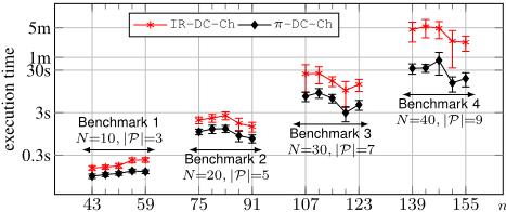
Both implementations were tested on instances of the four benchmarks from Hunsberger and Posenato [2016]. Each benchmark has at least 60 DC and 60 non-DC CSTNs, obtained from random workflow schemata generated by the ATAPIS toolset [Lanz and Reichert, 2014]. The numbers of activites (N) and observations (|P|) were varied, as shown in Fig. 4. Since non-DC networks were regularly solved one to two orders of magnitude faster than similarly sized DC networks, this section focuses on the results for the DC networks.

Fig. 4 displays the average execution times for the two algorithms over all four benchmarks, each point representing the average execution time for instances of the given size. We extended the benchmarks, adding up to 50 DC instances, to generate tight 95% confidence intervals. The results demonstrate that the 3-rule π-DC-Ch algorithm is much faster than the 6-rule IR-DC-Ch algorithm. Moreover, the performance improvement increases as the instance size increases.

Regarding non-DC networks, we verified that the difference in performance of the two algorithms is statistically insignificant: for each network size, the confidence intervals for the average execution times of the two algorithms invariably overlap.

6 Conclusions

This paper began by showing that the IR-DC semantics for CSTNs is flawed, and that one of the six rules from the IRDC-checking algorithm for CSTNs is unsound with respect to the IR-DC semantics. However, the major contribution of the paper was to present the simpler, three-rule π-DC-checking algorithm and prove that it is sound and complete with respect to the (unflawed) π-DC semantics from Cairo et al. [2016]. An empirical evaluation showed that the π-DC-checking algorithm is faster than the IR-DC-checking algorithm, which also happens to be sound and complete for the π-DC-checking problem.