
Non-decreasing Payment Rules for Combinatorial Auctions
Proceedings of the Twenty-Seventh International Joint Conference on Artificial Intelligence. Main track. Pages 105-113.
https://doi.org/10.24963/ijcai.2018/15
Keywords
- Agent-based and Multi-agent Systems: Algorithmic Game Theory
- Agent-based and Multi-agent Systems: Economic Paradigms, Auctions and Market-Based Systems
Abstract
Combinatorial auctions are used to allocate resources in domains where bidders have complex preferences over bundles of goods. However, the behavior of bidders under different payment rules is not well understood, and there has been limited success in finding Bayes-Nash equilibria of such auctions due to the computational difficulties involved. In this paper, we introduce non-decreasing payment rules. Under such a rule, the payment of a bidder cannot decrease when he increases his bid, which is a natural and desirable property. VCG-nearest, the payment rule most commonly used in practice, violates this property and can thus be manipulated in surprising ways. In contrast, we show that many other payment rules are non-decreasing. We also show that a non-decreasing payment rule imposes a structure on the auction game that enables us to search for an approximate Bayes-Nash equilibrium much more efficiently than in the general case. Finally, we introduce the utility planes BNE algorithm, which exploits this structure and outperforms a state-of-the-art algorithm by multiple orders of magnitude.
- [Baranov, 2010] Oleg Baranov. Exposure vs. free-riding in auctions with incomplete information. Technical report, Working paper, 2010.
- [Ausubel and Baranov, 2013] Lawrence Ausubel and Oleg Baranov. Core-Selecting Auctions with Incomplete Infor- mation. Working Paper, University of Maryland, Decem- ber 2013.
- [Ausubel and Baranov, 2017] Lawrence M Ausubel and Oleg Baranov. A practical guide to the combinatorial clock auction. The Economic Journal, 127(605), 2017.
- [Ausubel and Milgrom, 2006] Lawrence Ausubel and Paul Milgrom. The lovely but lonely Vickrey auction. In Peter Cramton, Yoav Shoham, and Richard Steinberg, editors, Combinatorial Auctions, pages 17-40. MIT Press, 2006.
- [Beck and Ott, 2013] Marissa Beck and Marion Ott. Incen- tives for overbidding in minimum-revenue core-selecting auctions. Working paper, Stanford University, 2013.
- [Bichler et al., 2014] Martin Bichler, Jacob Goeree, Stefan Mayer, and Pasha Shabalin. Spectrum auction design: simple auctions for complex sales. Telecommunications Policy, 38(7):613-622, 2014.
- [Bosshard et al., 2017] Vitor Bosshard, Benedikt Bünz, Ben- jamin Lubin, and Sven Seuken. Computing Bayes-Nash equilibria in combinatorial auctions with continuous value and action spaces. In Proceedings of the 26th Interna- tional Joint Conference on Artificial Intelligence (IJCAI), Melbourne, Australia, August 2017. IJCAI
- [Brown, 1951] George W Brown. Iterative solution of games by fictitious play. Activity Analysis of Production and Al- location, 13(1):374-376, 1951.
- [Clarke, 1971] Edward Clarke. Multipart pricing of public goods. Public Choice, 11(1):17-33, 1971.
- [Cramton et al., 2006] Peter Cramton, Yoav Shoham, and Richard Steinberg. Combinatorial Auctions. MIT Press, 2006.
- [Cramton, 2013] Peter Cramton. Spectrum auction design. Review of Industrial Organization, 42(2):161-190, 2013.
- [Day and Cramton, 2012] Robert W. Day and Peter Cram- ton. Quadratic core-selecting payment rules for combi- natorial auctions. Operations Research, 60(3):588-603, 2012.
- [Day and Milgrom, 2008] Robert W. Day and Paul Milgrom. Core-selecting package auctions. International Journal of Game Theory, 36(3):393-407, 2008.
- [Day and Raghavan, 2007] Robert W. Day and S. Ragha- van. Fair payments for efficient allocations in pub- lic sector combinatorial auctions. Management Science, 53(9):1389-1406, 2007.
- [Edelsbrunner et al., 1989] Herbert Edelsbrunner, Leonidas J Guibas, and Micha Sharir. The upper envelope of piecewise linear functions: algorithms and applications. Discrete & Computational Geometry, 4(4):311-336, 1989.
- [Goeree and Lien, 2016] Jacob Goeree and Yuanchuan Lien. On the impossibility of core-selecting auctions. Theoreti- cal Economics, 11:41-52, 2016.
- [Goetzendorff et al., 2014] Andor Goetzendorff, Martin Bichler, Robert Day, and Pasha Shabalin. Compact bid languages and core-pricing in large multi-item auctions. Management Science, 2014. Forthcoming.
- [Gretschko et al., 2016] Vitali Gretschko and Stephan Knapek and Achim Wambach. Strategic complexities in the combinatorial clock auction. Technical report, CESifo Working Paper No. 3983, 2016.
- [Groves, 1973] T. Groves. Incentives in teams. Economet- rica, 41(4):617-631, 1973.
- [Hartline et al., 2018] Jason Hartline, Nicole Immorlica, Mohammad Reza Khani, Brendan Lucier, and Rad Ni- azadeh. Fast core pricing for rich advertising auctions. In Proceedings of the 19th ACM Conference on Electronic Commerce (EC), 2018.
- [Karaca et al., 2018] O Karaca, P. G. Sessa, N. Walton, and M. Kamgarpour. Designing coalition-proof reverse auc- tions over continuous goods. Working Paper, ETH Zürich, 2018.
- [Lubin and Parkes, 2009] Benjamin Lubin and David Parkes. Quantifying the strategyproofness of mechanisms via metrics on payoff distributions. In Proceedings of the 25th Conference on Uncertainty in Artificial Intelligence (UAI), pages 349-358, 2009.
- [Lubin et al., 2018] Benjamin Lubin, Benedikt Bünz, and Sven Seuken. Designing core-selecting payment rules: A computational search approach. In Proceedings of the 19th ACM Conference on Electronic Commerce (EC), 2018.
- [Parkes et al., 2001] David C. Parkes, Jayant Kalagnanam, and Marta Eso. Achieving budget-balance with Vickrey- based payment schemes in exchanges. In Proceedings of the 17th International Joint Conference on Artificial Intel- ligence (IJCAI), Seattle, WA, August 2001.
- [Rabinovich et al., 2013] Zinovi Rabinovich, Victor Naro- ditskiy, Enrico H. Gerding, and Nicholas R. Jennings. Computing pure Bayesian-Nash equilibria in games with finite actions and continuous types. Artificial Intelligence, 195:106-139, 2013.
- [Reeves and Wellman, 2004] Daniel Reeves and Michael Wellman. Computing best-response strategies in infinite games of incomplete information. In Proceedings of the 20th Conference on Uncertainty in Artificial Intelligence (UAI), pages 470-478, 2004.
- [Sandholm, 2013] Tuomas Sandholm. Very-large-scale gen- eralized combinatorial multi-attribute auctions: Lessons from conducting $60 billion of sourcing. In Nir Vulkan, Alvin E. Roth, and Zvika Neeman, editors, The Handbook of Market Design, chapter 16. Oxford University Press, 2013.
- [Vickrey, 1961] William Vickrey. Counterspeculation, auc- tions, and competitive sealed tenders. The Journal of Fi- nance, 16(1):8-37, 1961.
References were extracted automatically from the PDF and may contain errors.
Full text extracted automatically from the PDF; figures, tables and equations may differ. The PDF is the version of record.
1 Introduction
Combinatorial auctions (CAs) are commonly used to allocate multiple, indivisible goods to multiple bidders. CAs allow bidders to express complex preferences on the space of all bundles of goods, taking into account that goods can be complements or substitutes [Cramton et al., 2006]. CAs have found widespread use in practice, including for the sale of radio spectrum licenses [Cramton, 2013], for the procurement of industrial goods [Sandholm, 2013], and for the allocation of TV ad slots [Goetzendorff et al., 2014].
Unfortunately, the incentive properties of CAs are not very well understood. One exception, of course, is the well-know VCG auction, which is strategyproof [Vickrey, 1961; Clarke, 1971; Groves, 1973]. However, using VCG in a CA domain can lead to undesirable outcomes, such as very low revenue [Ausubel and Milgrom, 2006] or collusion by bidders [Day and Milgrom, 2008].
1.1 Non-truthful Payment Rules
Due to VCG's shortcomings in CAs, non-truthful payment rules are used in practice. The most prominent among these are core-selecting payment rules [Day and Milgrom, 2008]. A rule is core-selecting if there is no group of bidders that is envious towards the auction winners. To achieve this, payments must lie in the core, which is the set of payments where no coalition of bidders is willing to pay more than what the auction charged the winners. The core is a convex polytope and the minimum revenue core is the face of the core where the total payment of all bidders is minimized. The VCGnearest payment rule (or "Quadratic"), the rule most often used in practice, selects the unique point in the minimum revenue core that minimizes the Euclidean distance to the VCG payment point [Day and Cramton, 2012]. To date, VCGnearest has been used in over ten spectrum auctions worldwide, generating more than $20 billion in revenues [Ausubel and Baranov, 2017]. Core-selecting CAs have also been proposed for use in electricity markets [Karaca et al., 2018] and in sponsored search auctions [Hartline et al., 2018]
Unfortunately, there does not exist a strategyproof coreselecting payment rule [Goeree and Lien, 2016], and relatively little is known about the incentives and strategic behavior of bidders when non-truthful payment rules like firstprice or core-selecting rules are used in CAs. Large settings with many bidders and goods are intractable to analyze, both analytically and computationally. Therefore, coreselecting CAs have mostly been analyzed in stylized settings [Ausubel and Baranov, 2013; Parkes et al., 2001]. Even so, many ways are known in which bidders can manipulate core-selecting CAs in their favor [Gretschko et al., 2016; Beck and Ott, 2013].
1.2 Background on BNE Algorithms
We employ the standard Bayes-Nash equilibrium (BNE) concept to analyze the incentives of bidders in a CA. A BNE, in contrast to the related Nash Equilibrium, captures the fact that bidders have incomplete information about their rivals' preferences. Bidders have a belief about other bidders' valuations, in the form of random variables drawn from the value space. Bidders submit their own bids, chosen from their action space, in response to the expected bids of others.
For the purpose of equilibrium computation, [Bosshard et al., 2017; Reeves and Wellman, 2004] have argued that CAs should be modeled as infinite games, i.e., games with continuous value and action spaces. The argument is that it is actually more difficult to compute equilibria for finite games with a large number of states than for infinite games. However, the infinite setting is very challenging in its own way: the BNE solution concept imposes an equilibrium condition on every valuation of every bidder simultaneously; thus, special care must be taken to ensure the equilibrium condition is met for all possible valuations. While it is possible to apply heuristics in this step (e.g. checking the equilibrium condition at a finite sample of valuations), such heuristic equilibria are difficult to interpret in a standard game-theoretic way. In contrast, the BNEs in the infinite game model are readily interpretable.
The state of the art in this area is the work of Bosshard et al. [2017], who describe a fast numerical algorithm for finding approximate BNEs (i.e. ε-BNEs) in the infinite setting. They also point out several pitfalls that should be avoided, under the label of the false precision problem, to ensure that the result of a search for ε-BNEs yields a correct ε.
The combinatorial nature of the problem, together with the incomplete information setting, make BNE computation a very hard, almost intractable problem. Even state-of-the-art algorithms can only solve instances of limited size. By size we mean the number of bidders and goods included in the auction, as well as the number of bundles each bidder bids on. The latter directly affects the dimensionality of bidders' strategies, because the bids on all different bundles must be jointly optimized by each bidder. Scalability in this dimension is thus particularly difficult.
Despite the high complexity of this problem, advances in algorithmic techniques for BNE computation can still be very beneficial. First, being able to quickly solve small-to-medium sized instances makes it possible to solve many of them, enabling approaches such as an algorithmic search for payment rules with desirable properties [Lubin et al., 2018]. Second, understanding small CA instances helps us develop a deeper understanding of the effects that drive strategic behavior in combinatorial auctions. For instance, the LLG domain has been extensively studied [Goeree and Lien, 2016; Beck and Ott, 2013; Ausubel and Baranov, 2013; Baranov, 2010], even though the only combinatorial interaction that arises is two local players needing to cooperate to jointly outbid the global player. There are many more interesting interactions that can already happen in domains such as LLLLGG [Bosshard et al., 2017], which have a size in-between very stylized/toy domains such as LLG and a fully fledged spectrum auction with hundreds of goods and dozens of bidders. With the advent of more efficient BNE algorithms, the possibility of systematically studying such domains is just beginning to open up.
1.3 Overview of our Contributions
In this paper, we aim to find new structural properties of CAs that help us better understand the strategic behavior of bidders in CAs and also allow us to design more effective BNE algorithms. This leads us to introduce and analyze non-decreasing payment rules for CAs. Such payment rules cannot decrease a bidder's payment when he increases his bid, unless the allocation changes. In Section 3, we introduce this property formally. We prove that VCG-nearest, the payment rule most commonly used in practice, is not non-decreasing. We also show that non-decreasing rules actually exist, by placing several well-known rules in this class, including strategyproof and core-selecting ones. In Section 4, we introduce a new algorithm to compute ε-BNEs that exploits the structure of non-decreasing payment rules. For this, we first show how piecewise constant strategies can be used as an auxiliary modeling step in the computation of ε-BNEs. Such strategies create a cell structure that helps us understand the combinatorial interactions when bids are multidimensional. Under a non-decreasing payment rule, this structure can be exploited to find the best response of a bidder to the strategies of all other bidders more efficiently. We assemble these ideas into the utility planes BNE algorithm which computes ε-BNEs for infinite games, while guaranteeing the correctness of ε. In Section 5, we evaluate the runtime of our algorithm in two different CA domains. We show that it outperforms the stateof-the-art algorithm by multiple orders of magnitude.
2 Formal Model
In this section, we introduce CAs with continuous values and bids. We use the well-known independent private values (IPV) model. In contrast to other work, we explicitly handle the occurrence of ties. This is necessary because we deal with piecewise constant strategies and thus cannot assume that ties will occur with probability 0, as would be the case with strictly monotone strategies.
2.1 Combinatorial Auctions
A combinatorial auction (CA) is a mechanism used to sell a set M = {1, 2, . . . ,m} of goods to a set N = {1, 2, . . . , n} of bidders. For each bundle of goods K ⊆ M, each bidder i has a value vi(K) ∈ R≥0, and submits a (possibly nontruthful) bid bi(K). We assume that each bidder only bids on a limited number of r bundles of interest (typically a true subset of all possible bundles). For a fixed r, the bid bi can thus be represented by a point in the action space Rr≥0 , with bids on all other bundles implicitly being 0. The bid profile b = (b1, . . . , bn) is the vector of all bids, and the bid profile of everyone except i is denoted b-i. The CA has an allocation rule X(b) which always produces an efficient allocation: it maximizes reported social welfare (the sum of all winning bids), by solving what is known as the winner determination problem. Bids can be such that ties occur, i.e. multiple allocations are efficient. Thus, X(b) is a correspondence (set-valued function), with each x ∈ X(b) having the same probability of being chosen. xi denotes the bundle assigned to i under allocation x, possibly the empty bundle. The CA also has a payment rule p(b, x) which is a function assigning a payment to each bidder based on the bid profile and allocation. We assume that the payment rule satisfies individual rationality, i.e. pi(b, x) ≤ bi(xi). Each bidder has a quasi-linear utility function ui(vi, b, x) = vi(xi) - pi(b, x). We also assume that the utility functions satisfy free disposal, i.e. a bidder always has weakly positive value for winning additional goods. 1
1 Formally, free disposal requires that for all K ⊆ K′ ⊆ M, we have that vi(K) ≤ vi(K′ ).
| bids {2} {1, | VCG | VCG-nearest | bids′ {2} {1, 2} | VCG′ | VCG-nearest′ | ||||
|---|---|---|---|---|---|---|---|---|---|
| Bidder #1 Bidder #2 Bidder #3 | {1} 4∗ 4∗ 2 2 | 2} 5 6 | 2 2 0 | 3 3 0 | {1} 4∗ 2 | 4∗ 2 | 7 6 | 3 2 0 | 3.5 2.5 0 |
2.2 CAs as Bayesian Games
We model the process of bidding in a CA as a Bayesian game. Each bidder knows his own valuation vi, but he only has probabilistic information (i.e. a prior) over each other bidder j's valuation vj, represented by the random variable Vj. The joint prior V = (V1, . . . , Vn) is common knowledge and consistent between bidders. We assume that the Vi are mutually independent. Each bidder chooses a strategy si. We assume that all strategies are pure, i.e. si is a function mapping values to bids. The expected utility of bidder i with value vi when bidding bi is given by
with the inner expectation corresponding to tie-breaking between efficient allocations. The amount of utility that a bidder i is "leaving on the table" when submitting bid bi (instead of bidding optimally) is called the utility loss, given by
The expected utility might be discontinuous and not have a maximum, which is why we take the supremum instead. Bidders are in an ε-equilibrium when the utility loss is small for all possible valuations of all bidders:
Definition 1. An ε-Bayes-Nash equilibrium (ε-BNE) is a strategy profile s∗ such that
3 Non-decreasing Payment Rules
In this section, we introduce non-decreasing payment rules. Informally, when a bidder increases his bid under such a rule, his payment cannot decrease unless the increased bid causes a change in the allocation. If the allocation stays fixed, then charging a smaller payment for a higher bid is counterintuitive. However, if the allocation changes, then it might very well be appropriate (in economic terms) to decrease the payment for a higher bid. For example, a bidder might currently be allocated the highly sought-after bundle K, and upon increasing his bid on a less-demanded bundle K′ , his allocation changes from K to K′ and his payment decreases.
Definition 2. For any allocation x, let Bx be the set of bid profiles for which x is efficient. The payment rule p(b, x) is non-decreasing at x if, for all bidders i and bid profiles b, b′ ∈ Bx with b-i = b′-i , the following holds:
A payment rule p(b, x) is non-decreasing if it is nondecreasing at all allocations x.
As we will show in Section 4, non-decreasing payment rules exhibit a particular structure that we can exploit in the design of BNE algorithms. However, this property is also desirable from an incentive point-of-view. Consider the strategyproof VCG payment rule, which is obviously nondecreasing, because under VCG, bidder i's payment is independent of his bid (and thereby also non-decreasing). Coupled with the welfare-maximizing allocation rule, this gives bidders an incentive to report their true valuations under VCG which leads to high efficiency. In contrast, a rule that is not a non-decreasing rule can be manipulated in surprising ways.
3.1 The VCG-nearest Rule
To illustrate this, consider the VCG-nearest payment rule. One justification for using this rule that has been provided in the literature is that VCG-nearest produces outcomes in the minimum revenue core and maximizes incentives for truthful bidding [Cramton, 2013; Day and Milgrom, 2008]. It is intuitive that minimizing the distance to VCG should reduce the "residual incentive to misreport" [Day and Cramton, 2012], but the evidence for this is sparse. Indeed, there are other ways to choose a minimum revenue core payment, and there is some evidence suggesting that VCG-nearest may not be the best [Lubin et al., 2018; Bichler et al., 2014].
As it turns out, VCG-nearest is not a non-decreasing payment rule, violating this property in many different situations. First, we discuss a simple example, which will also serve as proof for our claim.
Proposition 1. VCG-nearest is not non-decreasing.
Proof. Given by counterexample in Table 1, where bidder 2 decreases the payment on his winning bundle {2} by increasing his bid on losing bundle {1, 2} from 5 to 7.
Note that bidder 2 could also cause his payment to decrease by directly decreasing his bid on {2}. In contrast, the manipulation shown in Table 1 involves an over-bid, which can be particularly problematic for the auction process. The CCA, which is the auction format most often used in practice (e.g. for spectrum auctions) has a clock phase of several rounds used for price discovery, followed by a final round in which a sealed-bid CA is used. There are activity rules in place that force bidders to be consistent in their revealed preferences: their demand for goods must decrease in response to prices rising over time [Cramton, 2013]. The manipulation we show here allows bidder 2 to declare high demand for bundle {2} while keeping his anticipated payment low. This suggests that there may be ways to circumvent the activity rule by strategically exaggerating one's demand, a topic which should be investigated further.
| bundle of interest | bid | VCG | VCG-nearest | bid′ | VCG′ | VCG-nearest′ | |
|---|---|---|---|---|---|---|---|
| Bidder #1 | {1} | 5 | 2 | 37/12 | 5 | 1 | 36/12 |
| Bidder #2 | {2} | 5 | 0 | 16/12 | 5 | 0 | 18/12 |
| Bidder #3 | {3} | 4 | 1 | 37/12 | 5 | 1 | 36/12 |
| Bidder #4 | {4} | 1 | 0 | 7/12 | 1 | 0 | 6/12 |
| Bidder #5 | {5} | 1 | 0 | 7/12 | 1 | 0 | 6/12 |
| Bidder #6 | {6} | 1 | 0 | 10/12 | 1 | 0 | 12/12 |
| Bidder #7 | {1, 2, 4} | 5 | 5 | ||||
| Bidder #8 | {2, 3, 5} | 5 | 5 | ||||
| Bidder #9 | {1, 3, 6} | 7 | 7 | ||||
| Bidder #10 | {4, 5, 6} | 2 | 2 | ||||
| Bidder #11 | 3, | 5 | 5 |
{2, 3, 4}
Table 2: Auction where 11 single-minded bidders are bidding on 6 goods. We show VCG and VCG-nearest payments for each bidder. If bidder 3 increases his bid (marked in bold), this decreases bidder 1's VCG payment, which in turn decreases bidder 3's VCG-nearest payment.
This first counterexample already shows ways in which the VCG-nearest payment rule can be problematic. Unfortunately, there exist even more egregious cases. For instance, a bidder who is single-minded (i.e. who only bids on a single bundle) can sometimes decrease his payment by bidding higher on his bundle, even when he is already winning. VCGnearest is thus doing the direct opposite of what would be intuitive when receiving an economic signal of higher interest in a bundle.
Consider the situation in Table 2, where 11 bidders are bidding for 6 goods. We show two different bid profiles, along with the corresponding auction outcomes. The only difference between the bid profiles is that bidder 3 has increased his bid from 4 to 5, which causes bidder 1's VCG payment to drop from 2 to 1. In both situations, the winners are bidders 1-6, and each of the remaining bidders imposes a single core constraint. The minimum-revenue core is a line segment that fulfills all five of these constraints with equality, yielding a total payment of 9.5. However, bidder 3's payment under VCG-nearest decreases from 37/12 to 36/12.
3.2 Other Core-Selecting Payment Rules
We have already seen that VCG is non-decreasing, but it is not a core-selecting rule like VCG-nearest. Fortunately, many well-known core-selecting payment rules are also nondecreasing. This is straightforward to see for the first-price payment rule, which is non-decreasing because i's payment is directly proportional to the bid on the bundle he wins, and independent of his bids on other bundles. We now show that two other core-selecting rules are non-decreasing as well. The first one is the proportional rule, where the payments are on the core boundary and proportional to the winning bids. The second is the proxy rule, where we imagine a proxy agent bidding on behalf of each bidder in infinitesimal increments until a point in the core is hit [Ausubel and Baranov, 2013]. We provide formal definitions of these payment rules in Appendix A of the full version of this paper.
Proposition 2. The proportional and proxy rules are nondecreasing.
Proof. We show this for proportional, the argument is analogous for proxy. Let b and b′ be identical bid profiles, except for b′i (K) > bi(K), and let x be an allocation that is efficient under both b and b′ . There are three cases: (1) xi = ∅, thus i's payment is 0 by individual rationality. (2) xi = K. The core is the same w.r.t. b and b′ . Let ˜ p be the unique point on the line of payments proportional according to b′ with ˜ pi = pi(b, x). Since ˜ pj ≤ pj(b, x) ∀j ̸= i, ˜ p lies weakly below the core, thus pi(b′ , x) ≥ ˜ pi = pi(b, x). (3) xi = K′ ̸= K. Each core constraint under b′ is weakly higher than under b, but payments have the same proportion in both cases, so p(b, x) lies weakly below the core w.r.t. b′ . Thus pi(b′ , x) ≥ pi(b, x).
The intuition behind this proof is simple: Many coreselecting payment rules (such as proportional, proxy and vcgnearest) can be defined through the combination of a reference point and a method to project the payment to the core from the reference point [Lubin et al., 2018]. The core constraints themselves always increase in response to higher bids, and the reference point used for proxy and proportional is the origin. It is therefore sufficient to show that the projection method is non-decreasing, which is what the proof does.
The existence of payment rules which are both coreselecting and non-decreasing suggests re-evaluating the use of VCG-nearest in practice. Another payment rule may bring with it all the advantages of being in the core while being less manipulable and easier to work with for bidders and auctioneers. We leave a more detailed exploration of the space of non-decreasing core-selecting payment rules for future work.
4 The Utility Planes BNE Algorithm
In this section, we present our utility planes BNE algorithm, a highly efficient BNE algorithm for CAs with non-decreasing payment rules. We will make use of several building blocks. First, and most importantly, we will use an algorithmic trick, whereby our algorithm internally only considers piecewise constant strategies, i.e., strategies that consist of a finite number of flat segments. This will imply that only finitely many different bids can occur. This allows us to compute approximate best responses in a highly efficient manner using utility planes, as we will explain in Section 4.2. Note that if such a discretization were applied naively, this could lead to a phenomenon called the false precision problem [Bosshard et al., vi
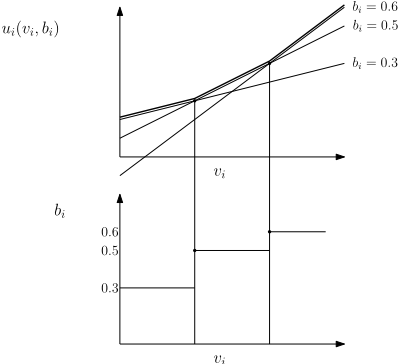
Figure 1: Example of utility planes in one dimension. Top: Each possible bid of a bidder generates a utility plane (a line in this case). The upper envelope is marked as a dashed line. Bottom: Piecewise constant strategy induced by the set of utility planes.
2017]. This problem arises when an auction game is simplified to make it tractable, an equilibrium is computed in the simplified game, and is then translated back to the original (richer) game without justification. This would lead to underestimating the potential utility loss and thus the ε in the computed equilibrium. Fortunately, the fact that we have nondecreasing payment rules allows us to use a powerful structural result (given as Theorem 1) to bound the utility loss, not only in relation to the restricted space of piecewise constant strategies, but with respect to all possible strategies. We provide details of this in Section 4.3. This enables us to avoid the false precision problem and compute a true ε-BNE of the original game. Our full BNE algorithm is presented in detail in Section 4.4.
4.1 Iterative Best Response Algorithms
Our BNE algorithm is based on the iterative best response paradigm. This is a well known approach to finding equilibria of games [Brown, 1951]. Starting at some strategy profile s, we repeatedly replace s with a best response to s, i.e. a strategy profile s′ where for each bidder i, strategy s′i maximizes his utility against the previous strategies s-i. While such algorithms usually have no convergence guarantees, they work well in practice and are robust to issues such as only having access to approximate best responses.
4.2 Computing Best Responses via Utility Planes
Recall that a strategy is a function mapping every valuation vi to a corresponding bid bi = si(vi). If we were to construct a best response to a strategy profile s naively, we would need to find a bid that maximizes the expected utility for each valuation vi separately. In fact, this is how Bosshard et al. [2017] compute best responses. They find the optimal bid for a finite number of valuations and then interpolate between these pointwise best responses to extend the strategy to the entire value space of the bidder. This "local" approach is straightforward but computationally expensive, because the expected utility must be computed for many (value, bid) pairs, without sharing any intermediate results between them.
Fortunately, two of our assumptions (quasi-linear utilities and independently distributed valuations) allow us to do better: we use a "global" approach, where we construct the best response strategy s′i without ever directly computing s′i (vi) for any particular vi. Note that for a fixed bid bi, the expected utility ¯ui(vi, bi) is linear in vi. Specifically, ¯ui contains one linear term for each bundle K, namely the value vi(K) times the probability of winning K. The remaining term is the expectation of -pi(b, x) across all bundles, which is constant in vi. Thus, ¯ui(vi, bi) forms a utility plane that maps valuations vi to expected utility [Rabinovich et al., 2013].
For a set of such utility planes, we can construct their upper envelope, which is a piecewise linear function defined as the pointwise maximum of all these planes (Figure 1, top). The value space is split into regions depending on which plane is the topmost one. This upper envelope naturally induces the best response, which is a piecewise constant strategy: for each region in the value space, the bid bi associated to the topmost plane is the one maximizing i's expected utility and is thus part of the best response (Figure 1, bottom).
The problem of computing upper envelopes is well known in computational geometry [Edelsbrunner et al., 1989]. In our implementation, we avoid constructing the envelope explicitly, because this is expensive and fraught with numerical precision issues. Instead, we evaluate the upper envelope for a finite set of valuations on a grid, and keep the strategy constant between grid points. This makes the best response less accurate, but only in a negligible way.
4.3 Partitioning the Action Space
Recall that the action space of bidder i is the set of all bids that i is allowed to submit, i.e. Rr≥0 , where r is the number of bundles of interest. We want to impose a structure on this space that will help us understand which bids we need to consider when computing the best response of i to some strategy profile s. This will also help us determine if s is an ε-BNE.
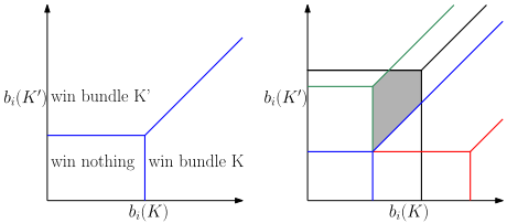
Consider the situation where the bids b-i of all other bidders are fixed. In this case, i's action space is partitioned into r + 1 convex polytopes, with i's allocation being different in each polytope (Figure 2, left). To explain how this partition arises, we need the concept of a constrained allocation rule. Recall that the allocation rule X(b) maximizes reported social welfare across all bidders. The constrained allocation rule X-i(K, b-i) also maximizes welfare, but is subject to the constraint that bundle K is allocated to bidder i. Thus, the total reported social welfare achieved by X-i(K, b-i) is a linear function of bi(K). Now, consider two bundles K and K′ . We can express the condition that X-i(K, b-i) achieves higher reported social welfare than X-i(K′ , b-i) as a linear inequality. Given a bid bi where i wins bundle K under the (unconstrained) efficient allocation, such a linear inequality must hold for every bundle K′ ̸= K. Thus, the set of all such bids forms a convex polytope.
Taking this idea further, if we have a probability distribution over finitely many bid profiles b-i (i.e. when each sj is a piecewise constant strategy), we can partition the action space of i into many smaller convex polytopes, such that inside each polytope, bidder i's probability of winning each bundle is the same (Figure 2, right). This finer partition can be visualized as intersecting the partitions corresponding to each possible b-i. We call each of these smaller polytopes a cell of bidder i's action space.
Next, we show that for any strategy profile s, we can bound the maximum utility that bidder i could possibly obtain by deviating from his current strategy. To compute this bound, we only need to consider what happens at all cell vertices. The idea is the following: if we have two different points bi ≤ b′i that are both strictly inside the same cell, then bidding bi is always preferable. This is because the non-decreasing payment rule ensures that the expected payment at bi is weakly lower than at b′i , while keeping the same distribution over allocations. Taking this idea to its logical conclusion, it is never optimal to bid anything other than the lowest vertex of a cell.
There is a catch, however: a vertex itself belongs to several cells, so bidding exactly on the vertex would lead to ties between different allocations for bidder i, making the auction result different from that of inner points of the cell. The optimal bid that is representative of a cell is thus strictly in the interior of the cell, just above the lowest vertex.
We cannot determine the payment for such an optimal bid exactly since we make no assumptions about the payment rule except that it is non-decreasing. 2 To solve this issue, we can compute the allocation as if i had bid sligthly above the vertex, but collect the payment as if he had bid exactly on the vertex. This results in an upper bound for the maximum utility that can be obtained anywhere in the cell in question. Formalizing the above, we introduce the tie-winning expected utility
where δ is a small constant, and the vector π corresponds to a permutation of (1, . . . , r) which moves the bid into one of the cells neighboring bi. The permutation π expresses some preference order over bundles in case of self-ties. Next, we introduce the i-optimal expected utility
2 In particular, the payment rule need not be continuous.
which maximizes over Π, the set of all such permutations. With this definition in place, we can state the main technical result of the paper.
Theorem 1. In a CA with a non-decreasing payment rule and where bidders have piecewise constant strategies, it holds that for every vi, there exists a cell vertex b∗i such that, for any bid bi in i's action space,
Proof. See Appendix B of the full version of this paper.
4.4 The Algorithm
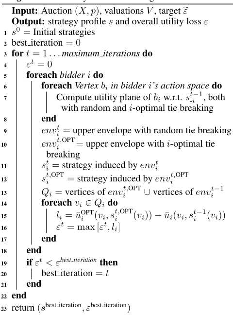
With Theorem 1, we now have all the pieces in place to build our algorithm. On a high level, our algorithm works as follows: We have a strategy profile s consisting of piecewise constant strategies. Thus, bidder i's action space has finitely many cell vertices and we can construct best response s′i from the utility planes corresponding to these vertices. s′i is an approximate best response over the full action space of i. The strategy profile s′ we construct in this way also consists of piecewise constant strategies, so we can repeat this procedure in the next iteration of our iterative best response algorithm.
Our full BNE algorithm is provided in Algorithm 1. The iterative best response loop is given in lines 3-22. In lines 6-8, we compute two sets of utility planes for each bidder: one for the actual expected utility ¯ui, and another for the ioptimal expected utility ¯uOPT i . In lines 9-10, we compute two upper envelopes, one for each set of utility planes. Line 11 computes bidder i's best response, i.e. the strategy obtaining the highest possible utility in response to st-1 -i . Line 12 computes the best response, assuming that i wins all ties and obtains the i-optimal utility. The utility loss of bidder i is calculated in lines 13-17 by comparing the utility obtained by the current strategy st-1 i to the utility obtained by the i-optimal best response at all vertices of both envelopes. In lines 19-21, we check if the strategy profile of the last iteration is a more accurate BNE than any previous strategy profile. The next theorem shows that Algorithm 1 computes a true ε-BNE:
Theorem 2. In a CA with a non-decreasing payment rule, Algorithm 1 returns strategy s and ε, such that s is an ε-BNE.
Proof. It follows from Theorem 1 that, for all vi, the envelope envt,OPT i (vi) is an upper bound for the utility obtainable at vi with any bid bi. For any two piecewise linear functions f and g, the maximum of the function h := g -f must occur at a vertex (one of the segment points) of either f or g. Both envt,OPT i and envt i are piecewise linear functions, and if we subtract themwe get an upper bound for the utility loss. It follows that εi computed in lines 14-17 of Algorithm 1 bounds the maximum utility loss of bidder i.
Discussion. With this theorem, our results are on solid ground: While our algorithm only considers a finite set of bids (because internally, it only operates with piecewise constant strategies), it measures the ε it achieves against the highest utility achievable by any bid, thus avoiding the false precision problem described by Bosshard et al. [2017].
The reason why our algorithm works well in practice also becomes clear now: the best responses we compute are almost optimal. In fact, a bidder loses very little utility by being restricted to bids that are cell vertices, namely the utility lost due to ties. This amount is very small when the grid resolution is large enough and value distributions are relatively close to uniform.
4.5 Runtime Analysis
Computing a utility plane is by far the most expensive part of Algorithm 1. Therefore, we evaluate its runtime in the unit cost model, counting the number of times this operation must be performed, and ignoring any other operations (e.g. the computation of the upper envelope).
The algorithm computes one utility plane for each vertex bi of the cell structure of bidder i. Luckily, the number of such vertices is bounded. If all strategies are piecewise constant, then we have a finite number of distinct bids used by each bidder. Thus, we can always find a step size such that any bid by any bidder on any bundle is an integer multiple of this step size. It turns out that if we build a regular grid with resolution equal to this step size and lay it over the action space of a bidder, then all cell vertices fall exactly on grid points.
Lemma 1. In a CA where bidders have piecewise constant strategies, if it is always the case that for some constant step size c ∈ R≥0, bi(K) is an integer multipe of c, then the coordinates of all cell vertices are also integer multiples of c.
Proof. Each cell vertex bi is defined by a linear system of equalities. The coefficients of these equalities are always 1, 0 or -1, so if we perform Gaussian elimination to find bi, we will add and subtract equations, but never multiply them. The claim easily follows from the fact that {a · c : a ∈ Z, c ∈ R} is closed under addition.
Lemma 1 allows us to bound the amount of work the algorithm does per iteration. If we choose the initial strategies to only contain bids on a regular grid, then the number of cell vertices does not grow over time, assuming that bidders never want to bid above their maximum value for any bundle. 3
For instance, if we have a bidder interested in two bundles with values in the [0, 2] interval, choosing a step size of c = 1/32 means that we need to compute at most 652 utility lines in each iteration. More generally, if a bidder has r bundles of interest, with each bundle Kj having value in the interval [0, vmax i (Kj)], then all vertices lie on an rdimensional grid with resolution c, going from 0 to vmax i (Kj) in each dimension. In that case we need to compute at most ( 1c +1)r · ∏rj=1 vmax i (Kj) utility lines for that bidder.
5 Experimental Results
In this section, we evaluate the performance of our utility planes BNE algorithm. We benchmark it against the algorithm from Bosshard et al. [2017] in two domains: the single-minded LLG domain and the multi-minded LLLLGG domain.
5.1 Experiment Setup
For each domain, we set a target ε. This target is 0.001 for LLG, and 0.02 for LLLLGG. For each algorithm, we measure the runtime required to reach a strategy profile that is proven to be an ε-BNE. The starting strategy profile is one where all bidders bid truthfully. 4
Both algorithms are written in Java 8 and share as much of their implementation as possible. There is often a need to integrate over the bids b-i, e.g. when computing expected utilities or utility planes. This integration is approximated using Monte Carlo sampling with common random numbers, as described in [Bosshard et al., 2017]. The number of samples used is 20,000 for LLG and 200,000 for LLLLGG.
3 For the first-price, proxy and proportional payment rules, we have found this to be the case in our experiments. Proving this property formally is an interesting open problem.
4 The cell structure we describe in Section 4.3 only arises when all bidders play piecewise constant strategies. Therefore, our BNE algorithm computes an inaccurate ε in the first iteration. To fix this issue, we make sure that the algorithm runs for at least two iterations.
| Domain & Rule | Runtime (Baseline) (Utility | Runtime Planes) | Speedup Factor |
|---|---|---|---|
| LLG (8 variations) | 0.0109 | 0.0017 | 6.45 |
| LLLLGG First Price | 151.30 | 1.75 | 86.45 |
| LLLLGG Proxy | 224.10 | 2.91 | 77.01 |
| LLLLGG Proportional† | 155.47 | 1.95 | 79.72 |
5.2 Local-Local-Global (LLG)
First, we consider the well-known LLG domain, a stylized setting with three bidders, two items and one bundle of interest per bidder. Bosshard et al. [2017] measure the average runtime of their BNE algorithm in 16 variations of this setting for which analytical BNEs are known and can be compared against [Ausubel and Baranov, 2013]. All of the payment rules used are non-decreasing, including VCG-nearest, which is non-decreasing in LLG, even if not in general. 8 of the 16 variations have independent bidder distributions. To achieve the required ε of 0.001, we employ 800 verification points for the baseline algorithm, and we compute 600 utility lines in our new algorithm.
Handling the Global Bidder. One peculiarity of LLG is that it is a dominant strategy for the global bidder to bid truthfully. This is easy to see, because from his perspective, a minimum revenue core-selecting auction is equivalent to a single item second price auction. This de facto reduces the game to two bidders. Unfortunately, our BNE algorithm requires all bidders to play piecewise constant strategies, so we cannot simply fix the global bidder to play the truthful strategy.
There are two possible ways to deal with this: the first option is to force the global bidder to play a piecewise constant strategy, and to include his utility loss in the computation of ε. The second option is to let the global bidder play truthfully, but bound the utility loss of the local bidders by pretending that the global bidder plays a piecewise constant strategy slightly above or below the truthful strategy.
We do the latter, to keep the runtime comparison between both algorithms as fair as possible. Specifically, when computing the actual utilities for the local bidders, we let the global bidder bid above truth, but when computing the ioptimal utilities, we let him bid below truth. In LLG, higher bids by the global bidder always lead to a decrease in the utilities of the local bidders. Our approach thus subtracts an underestimate of the utility obtained from an overestimate of the highest utility that could possibly be obtained. This produces a correct bound on the utility loss.
Results. The average runtimes are shown in the first row of Table 3. As one can see, our algorithm has much better performance than the baseline, leading to a speedup of 6.45x. Moreover, the equilibria we computed are close to the corresponding analytical BNEs: their L∞ distance is less than 0.043 in every case.
5.3 LLLLGG
Next, we test our algorithm in a larger setting, called LLLLGG. In this setting, we have 6 bidders and 8 items, with each bidder having two bundles of interest. The bidders are split into two classes: there are 4 local and 2 global bidders, with strategies being symmetric within each class. The value distributions of all bidders are independent of each other. For a detailed definition, see [Bosshard et al., 2017].
To compute ε-BNEs for this setting, we use a grid resolution of 1 32 . Since local bidders' values are drawn from [0, 1] and global bidders' values are drawn from [0, 2], we compute utility lines corresponding to 332 and 652 equally spaced bids, respectively. The baseline algorithm uses a grid of 1202 verification points for both the local and global bidders.
Results. We run experiments for three non-decreasing payment rules: First-price, proxy and proportional. The runtimes are shown in Table 3. 5 For all payment rules, the utility planes BNE algorithm finds a BNE over 77 times faster than the baseline.
6 Conclusion
In this paper, we have introduced non-decreasing payment rules, and we have shown that this property has important consequences for incentives and algorithm design. Importantly, the commonly used VCG-nearest rule is not nondecreasing and enables various kinds of manipulations. Our preliminary analysis suggests that rules that are not nondecreasing can be manipulated via overbidding. In contrast, we conjecture that overbidding is never favorable in CAs with non-decreasing payment rules. We have also developed the theory necessary to create the utility planes BNE algorithm, which exploits the structural properties of non-decreasing payment rules to search for ε-BNEs in a very efficient way. We have empirically found our algorithm to be highly performant, beating a recent state-of-the-art algorithm by multiple orders of magnitude. Thus, our BNE algorithm pushes the boundary on what problem sizes can be analyzed computationally when studying non-truthful payment rules for CAs. Overall, our results suggest that further analytical and algorithmic analysis of non-decreasing payment rules is a promising avenue for future research.
Acknowlegdements
This paper is partially based on work done by the second author for his master's thesis at ETH Z¨urich. We would like to thank our colleagues at ETHZ for making such collaborations possible.
†This rule did not converge in the baseline, only reaching ε = 0.026. We still include it in the runtime comparison.
5 The runtime of these three rules is orders of magnitudes faster than what Bosshard et al. [2017] reported for VCG-nearest in their paper. This is expected because VCG-nearest is very expensive to evaluate, needing to compute the VCG point and then solve a quadratic program [Day and Raghavan, 2007].
@inproceedings{ijcai2018p15,
  title     = {Non-decreasing Payment Rules for Combinatorial Auctions},
  author    = {Bosshard, Vitor and Wang, Ye and Seuken, Sven},
  booktitle = {Proceedings of the Twenty-Seventh International Joint Conference on
               Artificial Intelligence, {IJCAI-18}},
  publisher = {International Joint Conferences on Artificial Intelligence Organization},
  editor    = {Jérôme Lang},
  pages     = {105--113},
  year      = {2018},
  month     = {7},
  note      = {Main track},
  doi       = {10.24963/ijcai.2018/15},
  url       = {https://doi.org/10.24963/ijcai.2018/15},
}
TY - CPAPER TI - Non-decreasing Payment Rules for Combinatorial Auctions AU - Bosshard, Vitor AU - Wang, Ye AU - Seuken, Sven T2 - Proceedings of the Twenty-Seventh International Joint Conference on Artificial Intelligence, IJCAI-18 PB - International Joint Conferences on Artificial Intelligence Organization PY - 2018 SP - 105 EP - 113 DO - 10.24963/ijcai.2018/15 UR - https://doi.org/10.24963/ijcai.2018/15 ER -Copied
Machine-readable versions of this paper, for tools and AI agents:





