
nanoCoP: Natural Non-clausal Theorem Proving
Proceedings of the Twenty-Sixth International Joint Conference on Artificial Intelligence. Best Sister Conferences. Pages 4924-4928.
https://doi.org/10.24963/ijcai.2017/695
Keywords
- Artificial Intelligence: artificial intelligence
- Artificial Intelligence: knowledge representation and reasoning
Abstract
Most efficient fully automated theorem provers implement proof search calculi that require the input formula to be in a clausal form, i.e. disjunctive or conjunctive normal form. The translation into clausal form introduces a significant overhead to the proof search and modifies the structure of the original formula. Translating a proof in clausal form back into a more readable non-clausal proof of the original formula is not straightforward. This paper presents a non-clausal automated theorem prover for classical first-order logic. It is based on a non-clausal connection calculus and implemented with a few lines of Prolog code. Working entirely on the original structure of the input formula yields not only a speed up of the proof search, but the resulting non-clausal proofs are also shorter.
- [Andrews, 1981] Peter B. Andrews. Theorem proving via general matings. J. ACM, 28(2):193-214, 1981.
- [Antonsen and Waaler, 2007] Roger Antonsen and Arild Waaler. Liberalized variable splitting. J. Autom. Reason- ing, 38(1-3):3-30, 2007.
- [Beckert and Posegga, 1995] Bernhard Beckert and Joachim Posegga. leanTAP: Lean tableau-based deduction. J. Au- tom. Reasoning, 15(3):339-358, 1995.
- [Bibel, 1983] Wolfgang Bibel. Matings in matrices. Com- mun. ACM, 26(11):844-852, 1983.
- [Bibel, 1987] Wolfgang Bibel. Automated theorem proving. Artificial intelligence. F. Vieweg und Sohn, Wiesbaden, 2nd edition, 1987.
- [Eder, 1992] Elmar Eder. Relative Complexities of First Or- der Calculi. Vieweg, Braunschweig, 1992.
- [Frege, 1879] Gottlob Frege. Begriffsschrift: Eine der arithmetischen nachgebildete Formelsprache des reinen Denkens. L. Nebert, Halle, 1879.
- [Gentzen, 1935] Gerhard Gentzen. Untersuchungen über das Logische Schließen. Mathematische Zeitschrift, 39:176- 210, 405-431, 1935.
- [Hähnle et al., 2004] Reiner Hähnle, Neil. V. Murray, and Erik Rosenthal. Linearity and regularity with negation nor- mal form. Theoretical Computer Science, 328:325-354, 2004.
- [Hähnle, 2001] Reiner Hähnle. Tableaux and related meth- ods. In Alan Robinson and Andrei Voronkov, editors, Handbook of Automated Reasoning, volume I, chapter 3, pages 101-178. Elsevier Science B.V., 2001.
- [Issar, 1990] Sunil Issar. Path-focused duplication: A search procedure for general matings. In T. S. W. Dietterich, edi- tor, AAAI-90, pages 221-226. MIT Press, 1990.
- [Kaliszyk and Urban, 2015] Cezary Kaliszyk and Josef Ur- ban. FeMaLeCoP: Fairly efficient machine learning connection prover. In Martin Davis, Ansgar Fehnker, Annabelle McIver, and Andrei Voronkov, editors, LPAR- 20, volume 9450 of Lecture Notes in Artificial Intelligence, pages 88-96. Springer, 2015.
- [Kreitz and Otten, 1999] Christoph Kreitz and Jens Otten. Connection-based theorem proving in classical and non- classical logics. J. UCS, 5(3):88-112, 1999.
- [McCune, 2005] William McCune. Release of Prover9. 2005. Mile high conference on quasigroups, loops and nonassociative systems.
- [Otten and Bibel, 2003] Jens Otten and Wolfgang Bibel. leanCoP: lean connection-based theorem proving. Jour- nal of Symbolic Computation, 36(1-2):139-161, 2003.
- [Otten and Bibel, 2017] Jens Otten and Wolfgang Bibel. Ad- vances in connection-based automated theorem proving. In J. Bowen, M. Hinchey, and E.-R. Olderog, editors, Provably Correct Systems. Springer, 2017. [Otten, 2008] Jens Otten. leanCoP 2.0 and ileanCoP 1.2: High performance lean theorem proving in classical and intuitionistic logic. In Alessandro Armando, Peter Baum- gartner, and Gilles Dowek, editors, IJCAR 2008, volume 5195 of Lecture Notes in Artificial Intelligence, pages 283-291. Springer, 2008.
- [Otten, 2010] Jens Otten. Restricting backtracking in con- nection calculi. AI Commun., 23(2-3):159-182, 2010.
- [Otten, 2011] Jens Otten. A non-clausal connection calculus. In Kai Brünnler and George Metcalfe, editors, TABLEAUX 2011, volume 6793 of Lecture Notes in Artificial Intelli- gence, pages 226-241. Springer, 2011.
- [Otten, 2014] Jens Otten. MleanCoP: A connection prover for first-order modal logic. In Stéphane Demri, Deepak Kapur, and Christoph Weidenbach, editors, IJCAR 2014, volume 8562 of Lecture Notes in Artificial Intelligence, pages 269-276. Springer, 2014.
- [Otten, 2016] Jens Otten. nanoCoP: A non-clausal connec- tion prover. In Nicola Olivetti and Ashish Tiwari, editors, IJCAR 2016, volume 9706 of Lecture Notes in Artificial Intelligence, pages 302-312. Springer, 2016.
- [Plaisted and Greenbaum, 1986] David A. Plaisted and Steven Greenbaum. A structure-preserving clause form translation. J. Symbolic Computation, 2(3):293-304, 1986.
- [Reis, 2015] Giselle Reis. Importing SMT and connection proofs as expansion trees. In Proof Exchange for Theorem Proving (PxTP), volume 186 of EPTCS, pages 3-10, 2015.
- [Robinson and Voronkov, 2001] John Alan Robinson and Andrei Voronkov, editors. Handbook of Automated Rea- soning. Elsevier Science Publishers, Amsterdam, 2001.
- [Schmitt et al., 2001] Stephan Schmitt, Lori Lorigo, Christoph Kreitz, and Aleksey Nogin. JProver: Integrat- ing connection-based theorem proving into interactive proof assistants. In Rajeev Goré, Alexander Leitsch, and Tobias Nipkow, editors, IJCAR 2001, volume 2083 of Lecture Notes in Artificial Intelligence, pages 421-426.
- [Schulz, 2002] Stephan Schulz. E -a brainiac theorem prover. AI Commun., 15(2-3):111-126, 2002.
- [Stickel, 1988] Mark E. Stickel. A PROLOG technology the- orem prover: Implementation by an extended PROLOG compiler. J. Autom. Reasoning, 4(4):353-380, 1988.
- [Sutcliffe, 2009] Geoff Sutcliffe. The TPTP problem library and associated infrastructure: The FOF and CNF parts, v3.5.0. J. Autom. Reasoning, 43(4):337-362, 2009.
References were extracted automatically from the PDF and may contain errors.
Full text extracted automatically from the PDF; figures, tables and equations may differ. The PDF is the version of record.
1 Introduction
Automated Theorem Proving (ATP) in classical first-order logic is a core research area in the field of Automated Reasoning (see [Robinson and Voronkov, 2001] for an overview). It is concerned with the question whether a conjecture H is a logical consequence of a given set of axioms G1, . . . ,Gn, written G1, . . . ,Gn |= H, in which G1, . . . ,Gn,H are firstorder formulae. More specifically the objective in ATP is to find a proof for the validity of a given formula F. A formula F is valid if and only if it evaluates to true for all possible interpretation of its function and predicate symbols. According to the Deduction Theorem (for classical logic), G1, . . . ,Gn |= H holds if and only if there is a proof for the validity of the formula (G1 ∧ . . . ∧ Gn) ⇒ H. A formal description of the proof search algorithm is usually specified in form of a proof (search) calculus consisting of axioms and rules. Implementations of such proof calculi are called ATP systems or (automated theorem) provers.
Most efficient fully automated theorem provers implement proof calculi that require the input formula to be in a clausal form, i.e. disjunctive or conjunctive normal form. Formulae that are not in clausal form are translated into clausal form in a preprocessing step. For example, the formula F#
has the disjunctive normal form (quantifiers are eliminated)
While the use of a clausal form technically simplifies the proof calculi and their implementations, it has some fundamental disadvantages. The standard translation into clausal form as well as the definitional translation [Plaisted and Greenbaum, 1986; Eder, 1992], which introduces definitions for subformulae, cause a significant overhead for the proof search [Otten, 2010]. For example, the disjunctive normal form of F#, in which some parts of the formula are copied, has more than twice the size of the original formula. Furthermore, a translation into clausal form modifies the structure of the formula, hence, a translation of the clausal proof back into one of the original formula is not straightforward [Reis, 2015]. On the other hand, proof search with more "natural" non-clausal calculi, such as sequent or standard tableau calculi [Gentzen, 1935; H¨ahnle, 2001] is less efficient.
This paper describes the non-clausal prover nanoCoP for classical first-order logic [Otten, 2016]. By performing the proof search on the original structure of the input formula, it combines the advantages of more natural non-clausal calculi with the efficiency of a goal-oriented connection-based proof search. The prover is based on a non-clausal connection calculus [Otten, 2011] (Section 2) that generalizes the clausal connection calculus [Bibel, 1983; 1987] and is implemented in a very compact way (Section 3). It follows the lean methodology already used for the clausal connection prover leanCoP, whose minimal Prolog source code is shown in Figure 1. An experimental evaluation (Section 4) indicates a solid performance of nanoCoP.
prove(I,S):- \+member(scut,S) -> prove([-(#)],[],I,[],S) ; lit(#,C,_) -> prove(C,[-(#)],I,[],S). prove(I,S):- member(comp(L),S), I=L -> prove(1,[]) ; (member(comp(_),S);retract(p)) -> J is I+1, prove(J,S). prove([],_,_,_,_). prove([L|C],P,I,Q,S):- \+ (member(A,[L|C]), member(B,P), A==B), (-N=L;-L=N) -> ( member(D,Q), L==D ; member(E,P), unify_with_occurs_check(E,N) ; lit(N,F,H), (H=g -> true ; length(P,K), K<I -> true ; \+p -> assert(p), fail), prove(F,[L|P],I,Q,S) ), (member(cut,S) -> ! ; true), prove(C,P,I,[L|Q],S).2 The Non-clausal Connection Calculus
The standard notation for first-order formulae is used. Terms (denoted by t) are built up from functions (f, g, h, i), constants (a, b, c), and variables (x, y, z). An atomic formula (A) is built up from predicate symbols (P,Q,R, S) and terms; a (first-order) formula (F, G, H) is built up from atomic formulae, the connectives ¬, ∧, ∨, ⇒, and the first-order quantifiers ∀ and ∃. A literal L has the form A or ¬A. Its complement L is A if L is of the form ¬A; otherwise L is ¬L.
A term substitution σ assigns terms to variables. A formula in clausal form has the form ∃x1 . . . ∃xn(C1∨. . .∨Cn), where each clause Ci is a conjunction of literals L1, . . . , Lmi . It is represented as a set of clauses {C1, . . . ,Cn}, called a (clausal) matrix. A polarity 0 or 1 is used to represent negation, i.e. literals of the form A and ¬A are represented by A0 and A1 , respectively, A connection is a set {A0 , A1 } of literals with the same predicate symbol but different polarities.
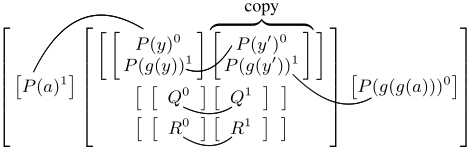
In a non-clausal matrix, a clause consists of literals and (sub)matrices. Let F be a formula and pol be a polarity. The non-clausal matrix M(F pol ) of a formula F pol is a set of clauses, in which a clause is a set of literals and matrices, and is defined according to Table 1. In Table 1, x∗ is a new variable, t∗ is the skolem term f ∗ (x1, . . . , xn) in which f ∗ is a new function symbol and x1, . . . , xn are the free variables in ∀xG or ∃xG. In G[x\t] all free occurrences of x in G are replaced by t. The non-clausal matrix M(F) of a formula F is the matrix M(F 0 ). In the graphical representation its clauses are arranged horizontally, while the literals and matrices of each clause are arranged vertically. For example, the formula F# of Section 1 has the simplified (i.e. redundant brackets are removed) non-clausal matrix M# =M(F#):
The graphical representation of the matrix M# is depicted in Figure 2. It already contains a clause copy with the fresh variable y′ and represents a non-clausal connection proof using the term substitution σ with σ(y) = a and σ(y′ ) = g(a); literals of each connection are connected with a line.
Compared to the formal clausal connection calculus [Otten and Bibel, 2003], a decomposition rule is added to the nonclausal calculus and the extension rule is slightly modified.
| type | F pol | M(F pol ) |
| atomic α | Apol (¬G)pol (G∧H)1 (G∨H)0 (G⇒H)0 (G∧H)0 (G∨H)1 | {{Apol }} M(G1-pol ) {{M(G1 )}, {M(H1 )}} {{M(G0 )}, {M(H0 )}} {{M(G1 )}, {M(H0 )}} {{M(G0 ),M(H0 )}} {{M(G1 ),M(H1 )}} {{M(G0 ),M(H1 )}} |
| β | (G⇒H)1 (∀xG)1 | M(G[x\x∗ ]1 ) |
| γ | (∃xG)0 (∀xG)0 (∃xG)1 | M(G[x\x∗ ]0 ) M(G[x\t∗ ]0 ) |
| δ | M(G[x\t∗ ]1 ) |
⎡⎢⎢⎢⎢⎣
⎤⎥⎥⎥⎥⎦
A clause C contains a literal L if and only if (iff) L∈C or C ′ contains L for M ′ ∈C, C ′∈M ′ . A clause C is α-related to a literal L iff it contains a matrix M ′ with {C ′ ,C ′′ }⊆M ′ for clauses C ′ ,C ′′ , such that C ′ contains L and C ′′ contains C (or C=C ′′ ). A copy of the clause C in the matrix M is made by renaming all free variables in C. M[C1\C2] denotes the matrix M, in which the clause C1 is replaced by C2. C ′ is a parent clause of C iff M ′ ∈C ′ and C ∈M ′ for some M ′ .
Let M be a matrix and Path be a set of literals. C is an extension clause (e-clause) of the matrix M with respect to a set of literals Path iff either (a) C contains a literal of Path, or (b) C is α-related to all literals of P ath occurring in M and if C has a parent clause, it contains a literal of Path. In the βclause of C2 with respect to L2, denoted by β-clauseL2 (C2), L2 and clauses that are α-related to L2 are deleted from C2.
The non-clausal connection calculus [Otten, 2011], which is sound and complete, is shown in Figure 3. Therein, M is a non-clausal matrix, C is a (subgoal) clause or ε (a special empty symbol) and (the active) Path is a set of literals or ε; σ is a term substitution. A non-clausal connection proof of M is a non-clausal connection proof of ε,M, ε.
The analytic, i.e. bottom-up, proof search is carried out in the same way as in the clausal calculus. Additional backtracking might be required when selecting C1 in the decomposition rule, but no backtracking is required when selecting M1. The rigid, i.e. single, term substitution σ is calculated whenever a connection is identified in a reduction or extension rule. On formulae in clausal form, the non-clausal connection calculus coincides with the clausal connection calculus.
| Axiom (A) | {},M, Path |
| Start (S) | C2,M, {} ε, M, ε and C2 is copy of C1∈M |
| Reduction (R) | C,M, Path∪{L2} C∪{L1},M, Path∪{L2} and σ(L1)=σ(L2) |
| Extension (E) | C3,M[C1\C2], Path∪{L1} C,M, Path C∪{L1}, M, P ath |
| and C3:=β-clauseL2 (C2), C2 is copy of C1, C1 is e-clause of M wrt. Path∪{L1}, C2 contains L2 with σ(L1)=σ(L2) | |
| Decomposition (D) | C ∪C1,M, Path C∪{M1},M, Path and C1∈M1 |
3 The nanoCoP TheoremProver
The implementation of the non-clausal connection calculus of Figure 3 follows the lean methodology [Beckert and Posegga, 1995], which is already used for the clausal connection prover leanCoP [Otten and Bibel, 2003]. It uses very compact Prolog code to implement the basic calculus and adds a few essential optimization techniques in order to prune the search space. The resulting natural nonclausal connection prover nanoCoP is available under the GNU General Public License and can be downloaded at http://www.leancop.de/nanocop/ .
In a first step, the input formula F is translated into a nonclausal (indexed) matrix M(F) according to Table 1; redundant brackets are removed [Otten, 2011]. Additionally, every (sub-)clause (I, V ) : C and (sub-)matrix J :M is marked with a unique index I or J; clause C is also marked with a set of variables V that are newly introduced in C but not in any subclause of C. Atomic formulae are represented by Prolog atoms, term variables by Prolog variables and the polarity 1 by "-". Sets, e.g. clauses and matrices, are represented by Prolog lists (representing multisets). For example, the matrix M# from Section 2 is represented by the Prolog term
[(0ˆK)ˆ[]:[-(p(a))], (1ˆK)ˆ[]:[2ˆK:[(3ˆK)ˆ[Y]:[p(Y),-(p(g(Y)))]], 4ˆK:[(5ˆK)ˆ[]:[q],(6ˆK)ˆ[]:[-q]], 7ˆK:[(8ˆK)ˆ[]:[r],(9ˆK)ˆ[]:[-r]]], (10ˆK)ˆ[]:[p(g(g(a)))]]in which the Prolog variable K is used to enumerate clause copies. In the second step, the matrix M =M(F) is written into Prolog's database. For every literal Lit in M the fact
lit(Lit,ClaB,ClaC,Grnd)is asserted into the database where ClaC ∈ M is the (largest) clause in which Lit occurs and ClaB is the β-clause of ClaC with respect to Lit. Grnd is set to g if the smallest clause in which Lit occurs is ground, i.e. does not contain any variables; otherwise Grnd is set to n. Storing literals of M in the database in this way is called lean Prolog technology [Otten, 2010] and integrates the advantages of the Prolog technology approach [Stickel, 1988] into the lean theorem proving framework. No other modifications or simplifications of the original formula are done during these two preprocessing steps.
The nanoCoP source code is shown in Figure 4. As an optimization, it uses positive start clauses [Otten, 2011], calculated by the predicate positiveC(Cla,Cla1).
The predicate prove(Mat,PathLim,Set,Proof) implements the start rule. Mat is the matrix generated in the preprocessing step, PathLim is the maximum size of the active path used for iterative deepening, and Proof contains the returned connection proof. Set is a list of options used to control the restricted backtracking technique [Otten, 2010] and may contain "cut" and "comp(I)" for I ∈IN. In order to achieve completeness, nanoCoP performs an iterative deepening on the size of the active path implemented within the second Prolog clause of this prove predicate.
The predicate prove(Cla,Mat,Path,PathI,PathLim, Lem,Set,Proof) implements the axiom, the decomposition rule, the reduction rule, and the extension rule of the non-clausal connection calculus of Figure 3. Cla, Mat, and Path represent the subgoal clause C, the (indexed) matrix M and the (active) Path. The term substitution σ is stored implicitly by Prolog. The indexed path PathI contains the indices of all clauses and matrices that contain literals of Path; it is used for calculating extension clauses. The list Lem is used for the lemmata rule and contains all literals that have already been "solved" [Otten, 2010]. This prove predicate succeeds iff there is a connection proof for the tuple Cla, Mat, Path with |Path|< PathLim. In this case Proof returns a connection proof. The input matrix Mat has to be stored in Prolog's database as explained above.
Finally, the last predicate prove_ec(ClaB,Cla1,Mat, PathI,ClaB1,Mat1) is used to calculate extension clauses. Starting with the (largest possible) extension clause Cla1, its β-clause ClaB, the current (indexed) matrix Mat, and the indexed path PathI, it returns an appropriate extension clause Cla, copies it into Mat and returns its β-clause ClaB1 and the new (indexed) matrix Mat1.
nanoCoP uses additional optimization techniques that are already used in the clausal connection prover leanCoP: regularity, lemmata, and restricted backtracking [Otten, 2010].
% start rule prove(Mat,PathLim,Set,[(Iˆ0)ˆV:Cla1|Proof]) :- member((Iˆ0)ˆV:Cla,Mat), positiveC(Cla,Cla1), prove(Cla1,Mat,[],[Iˆ0],PathLim,[],Set,Proof). prove(Mat,PathLim,Set,Proof) :- retract(pathlim) -> ( member(comp(PathLim),Set) -> prove(Mat,1,[],Proof) ; PathLim1 is PathLim+1, prove(Mat,PathLim1,Set,Proof) ) ; member(comp(_),Set) -> prove(Mat,1,[],Proof). % axiom prove([],_,_,_,_,_,_,[]). % decomposition rule prove([J:Mat1|Cla],MI,Path,PI,PathLim,Lem,Set,Proof) :- !, member(Iˆ_:Cla1,Mat1), prove(Cla1,MI,Path,[I,J|PI],PathLim,Lem,Set,Proof1), prove(Cla,MI,Path,PI,PathLim,Lem,Set,Proof2), append(Proof1,Proof2,Proof). % reduction and extension rules prove([Lit|Cla],MI,Path,PI,PathLim,Lem,Set,Proof) :- Proof=[[IˆV:[NegLit|ClaB1]|Proof1]|Proof2], \+ (member(LitC,[Lit|Cla]), member(LitP,Path), LitC==LitP), (-NegLit=Lit;-Lit=NegLit) -> ( member(LitL,Lem), Lit==LitL, ClaB1=[], Proof1=[] ; member(NegL,Path), unify_with_occurs_check(NegL,NegLit), ClaB1=[], Proof1=[] ; lit(NegLit,ClaB,Cla1,Grnd1), ( Grnd1=g -> true ; length(Path,K), K<PathLim -> true ; \+ pathlim -> assert(pathlim), fail ), prove_ec(ClaB,Cla1,MI,PI,IˆV:ClaB1,MI1), prove(ClaB1,MI1,[Lit|Path],[I|PI],PathLim,Lem,Set,Proof1) ), ( member(cut,Set) -> ! ; true ), prove(Cla,MI,Path,PI,PathLim,[Lit|Lem],Set,Proof2). % extension clause (e-clause) prove_ec((IˆK)ˆV:ClaB,IV:Cla,MI,PI,ClaB1,MI1) :- append(MIA,[(IˆK1)ˆV1:Cla1|MIB],MI), length(PI,K), ( ClaB=[JˆK:[ClaB2]|_], member(JˆK1,PI), unify_with_occurs_check(V,V1), Cla=[_:[Cla2|_]|_], append(ClaD,[JˆK1:MI2|ClaE],Cla1), prove_ec(ClaB2,Cla2,MI2,PI,ClaB1,MI3), append(ClaD,[JˆK1:MI3|ClaE],Cla3), append(MIA,[(IˆK1)ˆV1:Cla3|MIB],MI1) ; (\+member(IˆK1,PI);V\==V1) -> ClaB1=(IˆK)ˆV:ClaB, append(MIA,[IV:Cla|MIB],MI1) ).4 Experimental Evaluation
The following evaluations were conducted on a 3.4 GHz Xeon system with 4 GB of RAM running Linux 3.13.0 and ECLiPSe Prolog 5.10. The CPU time limit for all proof attempts was set 100 seconds.
The following formula Fn is a slightly extended version of the formula F# of Section 1, where f n , gn , hn , and in are abbreviations for n nested applications of these functions:
Table 2 shows the timings on this (valid) formula class for n=10, n=30, and n=90 for the following provers: the lean (non-clausal) tableau prover leanTAP [Beckert and Posegga, 1995], the resolution prover Prover9 [McCune, 2005], the superposition prover E [Schulz, 2002] (using options "--auto --tptp3-format"), the clausal connection prover leanCoP [Otten and Bibel, 2003; Otten, 2010], and nanoCoP. The leanCoP core prover with the standard ("[nodef]") and the definitional ("[def]") translation into clausal form were tested. For nanoCoP restricted backtracking was switched off (Set=[]). Times are given in seconds; the size of the returned proof tree, i.e. the number of nodes of the proof tree, is given in brackets.
The last line of Table 2 shows the number of proved problems of all 5051 first-order (FOF) problems in the TPTP library v3.7.0 [Sutcliffe, 2009]. For leanTAP, leanCoP, and nanoCoP, the required equality axioms were added in a preprocessing step (which is included in the timings). The nanoCoP core prover performs significantly better than both clausal form translations of the leanCoP core prover.
Furthermore, 40%/51% of the proofs found by nanoCoP are shorter than those of leanCoP [nodef]/[def], respectively; as many of the problems in the TPTP library are "mostly" in a clausal form, 56%/47% of the proofs have the same size. The proofs of nanoCoP are up to 96%/74% shorter than those of the leanCoP versions [nodef]/[def], respectively.
The "full" leanCoP 2.2 prover, which additionally uses a strategy scheduling [Otten, 2010], proves 1710 TPTP problems. The version of nanoCoP using a restricted backtracking strategy, i.e. Set=[cut,comp(6)], was tested as well; it proves 1485 TPTP problems.
Tests have also shown that the classical version of the non-clausal connection prover JProver [Schmitt et al., 2001], which is the only published non-clausal connection prover so far, has a lower performance than leanTAP.
| leanTAP 2.3 | Prover9 2009-02A | E 1.9 | leanCoP 2.2 [nodef] | [def] | nanoCoP [ ] | |
|---|---|---|---|---|---|---|
| F10 | 0.17 (128) | - | 1.22 (2916) | - | - | 0.09 (45) |
| F30 | - | - | 84.57 (57628) | - | - | 0.12 (125) |
| F90 | - | - | - | - | - | 0.42 (365) |
| TPTP | 404 | 1611 | 2782 | 1134 | 1065 | 1232 |
5 Conclusion
Formal reasoning is a fundamental task in mathematics, computer science and many related fields. Since Frege published the first formal calculus for first-order logic in his Begriffsschrift [Frege, 1879], the development and implementation of efficient proof calculi has made significant progress. But up to now, most -if not all- efficient fully automated theorem provers for classical first-order logic translate the input formula into a clausal form. By using the standard translation the size of the resulting formula can grow exponentially with respect to the size of the original formula. Even a definitional translation increases the size of the formula, which results in a significant overhead for the proof search [Otten, 2010]. Both clausal form translations modify the structure of the formula, making it difficult to translate the (clausal) proof back into a proof of the original formula.
This paper introduced nanoCoP, the first efficient nonclausal connection prover for classical first-order logic. Using non-clausal matrices the proof search works directly on the original structure of the input formula and, thus, avoids a translation into any clausal form. This combines the advantages of more natural non-clausal sequent or tableau provers with the goal-oriented efficiency of connection provers.
Even though the non-clausal inferences introduce a slight overhead, nanoCoP outperforms both clausal form translations of the leanCoP core prover on a large set of TPTP problems. About half of the returned non-clausal proofs are up to 96% shorter than their clausal counterparts.
nanoCoP returns a compact non-clausal connection proof. A connection corresponds to a closed branch in the tableau calculus [H¨ahnle, 2001] or an axiom in the sequent calculus [Gentzen, 1935]. Hence, the translation into, e.g., a sequent proof is straightforward. The compact size of nanoCoP makes it also a suitable tool for the development of verifiably correct software [Otten and Bibel, 2017], as its correctness can be proven much more easily than that of an ATP system consisting of several thousand lines of source code.
Only few research work investigates non-clausal connection calculi and implementations. Other approaches [Andrews, 1981; Bibel, 1987; H¨ahnle et al., 2004; Kreitz and Otten, 1999] work (efficiently) only for ground formulae or their implementation is not available anymore [Issar, 1990].
Another important application of nanoCoP is its usage within non-classical logics, such as (first-order) intuitionistic or modal logic, for which the use of a clausal form is either not desirable or not possible. Hence, future work includes the combination of the non-clausal approach with the prefix (unification) technique for some non-classical logics, as already done for leanCoP [Otten, 2008; 2014]. In order to improve performance, further optimization techniques need to be integrated into nanoCoP, such as strategy scheduling [Otten, 2010], learning [Kaliszyk and Urban, 2015] or variable splitting [Antonsen and Waaler, 2007].
Acknowledgements
The author would like to thank Wolfgang Bibel for his helpful comments on a preliminary version of this paper.
@inproceedings{ijcai2017p695,
  title     = {nanoCoP: Natural Non-clausal Theorem Proving},
  author    = {Otten, Jens},
  booktitle = {Proceedings of the Twenty-Sixth International Joint Conference on
               Artificial Intelligence, {IJCAI-17}},
  publisher = {International Joint Conferences on Artificial Intelligence Organization},
  editor    = {Carles Sierra},
  pages     = {4924--4928},
  year      = {2017},
  month     = {8},
  note      = {Best Sister Conferences},
  doi       = {10.24963/ijcai.2017/695},
  url       = {https://doi.org/10.24963/ijcai.2017/695},
}
TY - CPAPER TI - nanoCoP: Natural Non-clausal Theorem Proving AU - Otten, Jens T2 - Proceedings of the Twenty-Sixth International Joint Conference on Artificial Intelligence, IJCAI-17 PB - International Joint Conferences on Artificial Intelligence Organization PY - 2017 SP - 4924 EP - 4928 DO - 10.24963/ijcai.2017/695 UR - https://doi.org/10.24963/ijcai.2017/695 ER -Copied
Machine-readable versions of this paper, for tools and AI agents:





