
Self-Adjusting Memory: How to Deal with Diverse Drift Types
Proceedings of the Twenty-Sixth International Joint Conference on Artificial Intelligence. Best Sister Conferences. Pages 4899-4903.
https://doi.org/10.24963/ijcai.2017/690
Keywords
- Artificial Intelligence: machine learning
- Artificial Intelligence: artificial intelligence
- Artificial Intelligence: uncertainty in artificial intelligence
- Artificial Intelligence: other
Abstract
Data Mining in non-stationary data streams is particularly relevant in the context of the Internet of Things and Big Data. Its challenges arise from fundamentally different drift types violating assumptions of data independence or stationarity. Available methods often struggle with certain forms of drift or require unavailable a priori task knowledge. We propose the Self-Adjusting Memory (SAM) model for the k Nearest Neighbor (kNN) algorithm. SAM-kNN can deal with heterogeneous concept drift, i.e. different drift types and rates. Its basic idea are dedicated models for current and former concepts used according to the demands of the given situation. It can be robustly applied in practice without meta parameter optimization.
We conduct an extensive evaluation on various benchmarks, consisting of artificial streams with known drift characteristics and real-world datasets. Highly competitive results throughout all experiments underline the robustness of SAM-kNN as well as its capability to handle heterogeneous concept drift.
- [Arthur and Vassilvitskii, 2007] David Arthur and Sergei Vassilvitskii. k-means++: The Advantages of Careful Seeding. In Proceedings of the eighteenth annual ACM- SIAM symposium on Discrete algorithms, pages 1027- 1035. Society for Industrial and Applied Mathematics, 2007.
- [Atkinson and Shiffrin, 1968] Richard C Atkinson and Richard M Shiffrin. Human memory: A proposed system and its control processes. The psychology of learning and motivation, 2:89-195, 1968.
- [Atzori et al., 2010] Luigi Atzori, Antonio Iera, and Gia- como Morabito. The Internet of Things: A Survey. Com- puter networks, 54(15):2787-2805, 2010.
- [Bifet and Gavalda, 2007] Albert Bifet and Ricard Gavalda. Learning from Time-Changing Data with Adaptive Win- dowing. In SIAM International Conference on Data Min- ing (SDM), volume 7, page 2007. SIAM, 2007.
- [Bifet et al., 2010] Albert Bifet, Geoff Holmes, and Bern- hard Pfahringer. Leveraging Bagging for Evolving Data Streams. In Joint European Conference on Machine Learning and Knowledge Discovery in Databases, pages 135-150. Springer, 2010.
- [Bifet et al., 2013] Albert Bifet, Bernhard Pfahringer, Jesse Read, and Geoff Holmes. Efficient Data Stream Classifica- tion via Probabilistic Adaptive Windows. In Proceedings of the 28th Annual ACM Symposium on Applied Comput- ing, SAC '13, pages 801-806, New York, NY, USA, 2013. ACM.
- [Chen et al., 2014] M. Chen, S. Mao, and Y. Liu. Big data: A survey. Mobile Netw. and Appl., 19(2), 2014.
- [Ditzler et al., 2015] Gregory Ditzler, Manuel Roveri, Ce- sare Alippi, and Robi Polikar. Learning in nonstationary environments: A survey. Computational Intelligence Mag- azine, IEEE, 10(4):12-25, 2015.
- [Elwell and Polikar, 2011] R. Elwell and R. Polikar. In- cremental learning of concept drift in nonstationary en- vironments. IEEE Transactions on Neural Networks, 22(10):1517-1531, Oct 2011.
- [Gama et al., 2014] João Gama, Indrė Žliobaitė, Albert Bifet, Mykola Pechenizkiy, and Abdelhamid Bouchachia. A survey on concept drift adaptation. ACM Computing Surveys (CSUR), 46(4):44, 2014.
- [Jaber et al., 2013] Ghazal Jaber, Antoine Cornuéjols, and Philippe Tarroux. Online learning: Searching for the best forgetting strategy under concept drift. In Neural Informa- tion Processing, pages 400-408. Springer, 2013.
- [Kolter and Maloof, 2007] J Zico Kolter and Marcus A Mal- oof. Dynamic weighted majority: An ensemble method for drifting concepts. The Journal of Machine Learning Research, 8:2755-2790, 2007.
- [Losing et al., 2016] V. Losing, B. Hammer, and H. Wers- ing. Knn classifier with self adjusting memory for hetero- geneous concept drift. In 2016 IEEE 16th International Conference on Data Mining (ICDM), pages 291-300, Dec 2016.
- [Losing et al., 2017] Viktor Losing, Barbara Hammer, and Heiko Wersing. Tackling Heterogeneous Concept Drift with the Self Adjusting Memory (SAM). Knowledge and Information Systems (under review), 2017.
- [Oza, 2005] Nikunj C. Oza. Online Bagging and Boost- ing. In IEEE International Conference on Systems, Man and Cybernetics 2005, volume 3, pages 2340-2345. IEEE, 2005.
- [Schiaffino et al., 2008] Silvia Schiaffino, Patricio Garcia, and Analia Amandi. eTeacher: Providing personalized as- sistance to e-learning students. Computers & Education, 51(4):1744-1754, 2008.
References were extracted automatically from the PDF and may contain errors.
Full text extracted automatically from the PDF; figures, tables and equations may differ. The PDF is the version of record.
1 Introduction
The classical batch setting of machine learning assumes that the complete task-specific data is all time available and can be accessed simultaneously without any restriction regarding the processing time. Furthermore, it is premised that the data is independent and identically distributed (i.i.d.). State of the art machine learning methods are able to obtain very accurate results within this framework. However, an ever growing field of real-world applications generates data in streaming fashion at increasing rate, requiring large-scale and real-time processing as well as life-long learning. Streaming data is prevalent in domains such as health monitoring, traffic management, financial transactions, social networks [Chen et al., 2014] and is the foundation of the Internet of Things [Atzori et al., 2010] technology. Supplementing streaming data with non-stationary environments leads to one of the recent key areas in data mining research: Learning in streams under concept drift. Here, algorithms are challenged by a variety of possible forms of drift under strict limitations in terms of memory consumption and processing time.
Heiko Wersing
HONDA Research Institute Europe Carl-Legien-Str. 30, 63073 Offenbach amMain
heiko.wersing@honda-ri.de
In supervised classification, concept drift [Gama et al., 2014] occurs when the joint distribution between the set of features x ∈ Rn and the target variable y ∈ {1, . . . , c} changes for at least two time steps t0 and t1:
The term real drift is used to specify that the relation between observation and labels Pt(y|x) varies over time. Virtual drift is present when the feature distribution Pt(x) changes without affecting the posterior of the classes Pt(y|x). Furthermore, the rate at which drift is taking place can be either classified as abrupt, resulting in a severe shift within the distribution, e.g. caused by a malfunctioning sensor, or incremental, an evolving change over time, e.g. evoked by a slowly degrading sensor. In the context of seasonal effects, drift is often characterized as reoccurring to describe that previous concepts are repeatedly emerging. In recent years, a few algorithms have been published which can be roughly divided in active and passive approaches [Ditzler et al., 2015]. Due to space constraints, we primarily review methods that are later also used in the experiments. A more complete overview is given in [Gama et al., 2014].
Active approaches explicitly detect the time of change and usually discard the accumulated knowledge up to this point. Often statistics such as the classification error, calculated on different time periods, are analyzed for significant deviations. A popular representative of these methods is ADaptive sliding WINdowing (ADWIN) [Bifet and Gavalda, 2007], utilized in various published algorithms. It efficiently monitors the binary error history since the last detected change. The history is repeatedly partitioned into two windows of various size. Whenever the difference of their average error exceeds a threshold a change is detected and the older window is dropped. Active approaches are often combined with a sliding window containing the most recent examples, as these are assumed to be the most valuable for current predictions. Hereby, the size is a trade-off between fast adaptation (small window) and good generalization in stable phases without drift (large window). To achieve both properties at the same time the size is adjusted dynamically. One exemplary method is the Probabilistic Adaptive Windowing (PAW) [Bifet et al., 2013] which randomly removes examples from the sliding window leading to a mix of recent and older instances. Active methods are able to quickly detect abrupt drift, however, they struggle with incremental change, which may not be significant enough and remains undetected. Another weakness is that knowledge either slowly fades out or is discarded in case of detected drift. Although the most recent examples are usually the most valuable for current predictions, there are also cases in which older data carries crucial information, e.g. reoccurring drift.
Passive approaches continuously adapt their model without explicit awareness of occurring drift. This prevents pitfalls such as missed or false detected drifts on the one hand, but the adaption speed is more or less constant, leading to costly delays in the case of abrupt drift, on the other hand. Passive algorithms are dominated by ensembles whose members are updated with incoming examples using techniques such as Bagging or Boosting. Jaber et al. presented Dynamic Adaption to Concept Changes (DACC) in [Jaber et al., 2013], an algorithm inspired by the Dynamic Weighted Majority [Kolter and Maloof, 2007] method. A classifier of the worst half of the pool is randomly removed after a predefined number of examples and replaced by a new one. Predictions for incoming examples are solely done by the best classifier within the pool, having the highest accuracy in the past. In Leveraging Bagging (LVGB) [Bifet et al., 2010] the randomization of Online Bagging [Oza, 2005] is increased and thereby also the diversity of the resulting ensemble. Additionally, ADWIN is used as change detector for every ensemble member such that every detected change leads to the replacement of the worst classifier by a new one. Learn++.NSE [Elwell and Polikar, 2011] processes incoming examples in chunks with a predefined size. A base classifier is trained for each chunk and added to the ensemble. In contrast to other methods, members are not learning continuously, but preserve their initial state. This fact is used to revive former members in the presence of reoccurring drift. Passive approaches can deal with incremental drift, but their inherent adaption speed has to be adjusted to the task-specific drift speed. In case of abrupt drift, the adaption delay is usually more pronounced than into active methods.
Even though some of the introduced methods can be used for several types of drift by an appropriate setting of their meta parameters, this requires explicit prior knowledge about the task at hand. However, it is still unclear how to identify the type of drift in a given real-world data stream. Furthermore, in real-world applications, data usually do not change only in one specific form, but instead multiple, sometimes even concurrent, types of drift are taking place at various rates. One example is the field of personalized assistance, in which individual user behavior is taken into account to provide appropriate assistance in various situations [Schiaffino et al., 2008]. But, individual behavior in particular can change in arbitrary ways. Systems anticipating only certain forms of drift, will perform sub-optimal at best, or fail completely at worst, when unexpected forms of change occur.
Our Self-Adjusting Memory (SAM) in combination with the k Nearest Neighbor (kNN) classifier is able to cope with heterogeneous concept drift and can be easily applied in practice without any parametrization. The extensive evaluation on common benchmarks demonstrates the gain of SAM-kNN in comparison to current state of the art approaches. It exclusively achieves highly competitive results throughout all experiments, demonstrating its robustness and the capability of handling heterogeneous concept drift. This paper is an abridged report of [Losing et al., 2016].
2 Streaming Setting
Our focus is data stream classification under supervised learning for incremental / on-line algorithms. A potentially infinite sequence S = (s1, s2, . . . , st, . . .) of tuples si = (xi, yi) arrives one after another. As t represents the current time stamp, the learning objective is to predict the target variable yt ∈ {1, . . . , c} for a given set of features xt ∈ Rn . The prediction ˆ yt = ht-1(xt) is done according to the previously learned model ht-1. Before proceeding with the next example, the learning algorithm generates a new model ht = train(ht-1, st) based on the current tuple st and the previous model ht-1. The performance is measured via the Interleaved Test-Train error E(S) = 1t ∑ti=1 1(hi-1(xi) ̸= yi).
3 Architecture of SAM
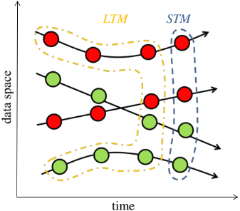
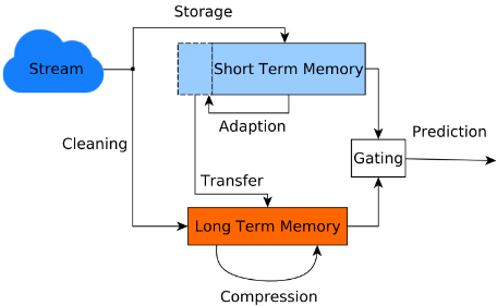
In the research field of human memory the dual-store model [Atkinson and Shiffrin, 1968], consisting of the Short-Term and Long-Term memory (STM & LTM), is largely accepted. The SAM architecture is partly inspired by this model and exhibits analogies such as the explicit separation of current and past knowledge, different conservation spans among the memories, filtered transfer of knowledge from the STM to the LTM as well as a situation dependent usage of both memories.
Our basic idea is to combine dedicated models for the current concept Pt(x, y) and all former ones Pt-1(x, y), . . . , P1(x, y) in such a way that the prediction error is minimized. We construct two different memories: The Short-Term Memory (STM), containing data of the current concept and the Long-Term Memory (LTM), maintaining knowledge of past concepts. This approach is illustrated by Figure 1. We share the general assumption of new data being more relevant for current predictions. Hence, we remove those information from former concepts which is in conflict with the current one, but we explicitly preserve the rest in compressed fashion. We avoid any parametrization, by exploiting the minimization of the error on recent data at various steps. Our architecture is depicted in Figure 2 and described below in detail.
3.1 Model Definition
Memories are represented by sets MST, MLT, MC. Each memory is a subset in Rn × {1, . . . , c} of varying length, adjusted during the adaptation process. The STM represents the current concept and is a dynamic sliding window containing the most recent m examples of the data stream:
The LTM preserves all former information which is not contradicting those of the STM in a compressed way. In contrast to the STM, the LTM is neither a continuous subpart of the stream nor given by exemplars, but instead a set of p points:
The combined memory (CM) is the union of both memories with size m + p and defined as MC = MST ∪ MLT.
Every set induces a classifier, in our case a distance weighted kNN : Rn ↦→ {1, . . . , c}, kNNMST , kNNMLT , kNNMC . Weights wST, wLT, wC are representing the accuracy of the corresponding model on the current concept and are determined as described in section 3.2. The prediction of our complete model relies on the sub-model with the highest weight and is defined for a given point x as:
This model is adapted incrementally for every time t as described in section 3.2.
The hyperparameters of the model consist of the minimal length of the STM Lmin, the maximum number of stored examples Lmax (STM & LTM combined) as well as the number of neigbhors k. These can be robustly chosen and do not require a task-specific setting 1 .
3.2 Model Adaption
The adaption comprises the size m of the STM, the data points in the LTM and the weights wST, wLT, wC of the corresponding sub-models.
Adaption of the short termmemory
The STM is a dynamic sliding window containing the most recent examples. Every incoming example of the stream gets inserted such that the STM grows continuously. Its role is to exclusively contain data of the current concept. Therefore, its size has to be reduced, whenever the concept changes such that examples of the former concept are dropped. However, we do not explicitly detect a concept change, but instead we adjust the size such that the Interleaved Test-Train error of the remaining STM is minimized. This approach relies on the fact that a model trained on internally consistent data yields less errors and we assume the remaining instances to represent the current concept or being sufficiently "close" to it.
We evaluate differently sized STMs and adopt the one with minimum error for MSTt+1 . We test only bisected window sizes to bound logarithmically the number of comparisons. Whenever the STM is shrunk, the set of discarded examples Ot is defined as
Cleaning and transfer
The LTM contains all data of former concepts that is consistent with the STM. This requires a cleaning of the LTM according to every seen example. In addition, whenever the STM is reduced in size, we do not simply discard the data sorted out, since it still may contain valuable information for future prediction. One example for such a situation is reoccurring drift, as methods preserving knowledge in this case do not have to relearn former concepts and therefore produce fewer errors. Instead, we transfer as much knowledge as possible into the LTM. Before doing so, we delete examples from the separated set Ot (see eq. 1) which are contradicting those in MSTt+1 . This adaption is formalized by two operations.
- We clean a set A by another set B regarding an example (xi, yi) ∈ B
where A,B, ˆ A ⊂ Rn × {1, . . . , c} and (xi, yi) ∈ B. ˆ A is defined in two steps.
(1) We determine the k nearest neighbors of xi in B \ (xi, yi) and select the ones with label yi. These define the threshold
(2) The k nearest neighbors of xi ∈ A which are inconsistent to B are cleaned based on the threshold, yielding the result of this operation:
1 We used for all experiments k = 5, Lmin = 50, Lmax = 5000.
2. We also require a cleaning operation for the full set B
where A,B, ˆ A|B| ⊂ Rn × {1, . . . , c}. This is defined iteratively by applying the former cleaning for all (xi, yi) ∈ B = {(x1, y1), . . . , (x|B|, y|B|)} as
The adaption of the LTM takes place at two different steps. To ensure a consistent model at any time, cleaning takes place according to every incoming sample (xt, yt)
Whenever the STM is shrunk, the discarded set Ot is transferred into the LTM after cleaning, i.e. the LTM becomes
Compression of the long termmemory
In contrast to the FIFO principle of the STM, instances are not fading out as soon as the size limit of the LTM is reached. Instead, we condense the available information to a sparse knowledge representation via clustering. This enables a far longer conservation than possible with simple out fading. Formally, for every class label ˆ c we group the corresponding data points in the LTM as MLTˆ c = {xi|(xi, ˆ c) ∈ MLT}. We use the clustering algorithm kMeans++ [Arthur and Vassilvitskii, 2007] with |MLTˆ c |/2 clusters. The resulting prototypes ˆMLTˆ c represent the compressed original data. The LTM is given by the union of all prototypes
This process is repeated each time the size limit is reached leading to a self-adapting level of compression.
Model weight adaption
The weight of a memory is its accuracy averaged over the last mt samples, where mt = |MSTt | is the size of the current STM. Hence, the weight of the LTM at time stamp t equals
and analogous for STM and CM.
4 Experiments
We couple the SAM architecture with the kNN classifier and evaluate it in comparison to well-known state of the art algorithms for handling concept drift in streaming data. Next to the methods discussed in section 1, we compare against a kNN classifier with a sliding window of fixed size (kNNS). A rough taxonomy of the methods is depicted in Table 1. The evaluation was done with common artificial and real-world benchmarks, which are extensively described in [Losing et al., 2016]. Window based approaches were allowed to store up to 5000 samples but never more than 10% of the whole dataset. No dataset specific hyperparameter tuning was done.
| L++.NSE | DACC | LVGB | kNNS | PAW | SAM | |
|---|---|---|---|---|---|---|
| Drift handling Classifier Ensemble | passive Decision tree 3 | passive Decision tree 3 | active Decision tree 3 | passive kNN 7 | active kNN 7 | passive kNN 3 |
| Table 2: | Error rates | of all experiments. |
| Dataset | Drift properties | L++.NSE | DACC | LVGB | kNNS | PAW | SAM |
|---|---|---|---|---|---|---|---|
| SEA Concepts | abrupt real | 14.48 | 15.68 | 11.69 | 13.83 | 13.39 | 12.50 |
| Rotating Hyperplane | incremental real | 15.58 | 18.20 | 12.53 | 16.00 | 16.16 | 13.31 |
| Moving RBF | incremental real | 44.50 | 54.34 | 44.84 | 20.36 | 24.04 | 15.30 |
| Interchanging RBF | abrupt real | 27.52 | 1.40 | 6.11 | 45.92 | 8.56 | 5.70 |
| Moving Squares | incremental real | 65.90 | 1.17 | 12.17 | 68.87 | 61.01 | 2.30 |
| Transient Chessb. | abr. reoc. virtual | 1.98 | 43.21 | 17.95 | 7.36 | 14.44 | 6.25 |
| Mixed Drift | various real/virtual | 40.37 | 61.06 | 26.29 | 31.00 | 26.75 | 13.33 |
| Artificial ∅ | 30.05 | 27.87 | 18.80 | 29.05 | 23.48 | 9.81 | |
| Artificial ∅ Rank | 4.00 | 4.57 | 2.86 | 4.29 | 3.57 | 1.71 | |
| Weather | virtual | 22.88 | 26.78 | 21.89 | 21.53 | 23.11 | 21.74 |
| Electricity | real | 27.24 | 16.87 | 16.78 | 28.61 | 26.13 | 17.52 |
| Cover Type | real | 15.00 | 10.05 | 9.07 | 4.21 | 6.76 | 4.8 |
| Poker Hand | virtual | 22.14 | 20.97 | 13.65 | 17.08 | 27.94 | 18.45 |
| Outdoor | virtual | 57.80 | 35.65 | 39.97 | 13.98 | 16.30 | 11.25 |
| Rialto | virtual | 40.36 | 28.93 | 39.64 | 22.74 | 24.96 | 18.58 |
| Real-world ∅ | 30.90 | 23.21 | 23.50 | 18.03 | 20.87 | 15.40 | |
| Real-word ∅ Rank | 5.33 | 4.17 | 3.17 | 2.33 | 4.00 | 2.00 | |
| Overall ∅ | 30.44 | 25.72 | 20.97 | 23.96 | 22.27 | 12.39 | |
| Overall ∅ Rank | 4.62 | 4.38 | 3.00 | 3.38 | 3.77 | 1.85 |
The error rates of all experiments are shown in Table 2 1 . SAM significantly outperforms the others by having nearly half the error rate in average compared to the second best method LVGB. Even more important is the fact that whereas other methods struggle at some datasets our approach delivers robust results without any hiccup. All concept drift types are handled better or at least competitive. Our results confirm the fact that kNN is in general a very competitive algorithm in the streaming setting. It is quite surprising that the simple sliding window approach kNNS performs comparably well or even better than more sophisticated methods such as DACC or L++.NSE. A more detailed evaluation as well as an analysis of the memory behavior and their respective functions can be found in [Losing et al., 2016].
5 Conclusion
In this paper we presented the Self-Adjusting Memory (SAM) architecture, especially designed to handle heterogeneous concept drift within streaming data. It explicitly separates the current concept from former ones and preserves both in dedicated memories. Thereby, it omits a common weakness of available methods which simply discard former knowledge and, therefore, have to relearn concepts in case of reoccurring concept drift. Our method is easy to use in practice since it requires no task-specific meta-parameterization. We compared SAM with current state of the art methods on various artificial and real-world benchmarks. As the only algorithm it demonstrated consistently accurate results for heterogeneous concept drift.
1 The drift properties of the real-world data were determined as described in [Losing et al., 2017]
@inproceedings{ijcai2017p690,
  title     = {Self-Adjusting Memory: How to Deal with Diverse Drift Types},
  author    = {Losing, Viktor and Hammer, Barbara and Wersing, Heiko},
  booktitle = {Proceedings of the Twenty-Sixth International Joint Conference on
               Artificial Intelligence, {IJCAI-17}},
  publisher = {International Joint Conferences on Artificial Intelligence Organization},
  editor    = {Carles Sierra},
  pages     = {4899--4903},
  year      = {2017},
  month     = {8},
  note      = {Best Sister Conferences},
  doi       = {10.24963/ijcai.2017/690},
  url       = {https://doi.org/10.24963/ijcai.2017/690},
}
TY - CPAPER TI - Self-Adjusting Memory: How to Deal with Diverse Drift Types AU - Losing, Viktor AU - Hammer, Barbara AU - Wersing, Heiko T2 - Proceedings of the Twenty-Sixth International Joint Conference on Artificial Intelligence, IJCAI-17 PB - International Joint Conferences on Artificial Intelligence Organization PY - 2017 SP - 4899 EP - 4903 DO - 10.24963/ijcai.2017/690 UR - https://doi.org/10.24963/ijcai.2017/690 ER -Copied
Machine-readable versions of this paper, for tools and AI agents:





