
Order Statistics for Probabilistic Graphical Models
Proceedings of the Twenty-Sixth International Joint Conference on Artificial Intelligence. Main track. Pages 4625-4631.
https://doi.org/10.24963/ijcai.2017/645
Keywords
- Uncertainty in AI: Approximate Probabilistic Inference
- Uncertainty in AI: Graphical Models
Abstract
We consider the problem of computing r-th order statistics, namely finding an assignment having rank r in a probabilistic graphical model. We show that the problem is NP-hard even when the graphical model has no edges (zero-treewidth models) via a reduction from the partition problem. We use this reduction, specifically a pseudo-polynomial time algorithm for number partitioning to yield a pseudo-polynomial time approximation algorithm for solving the r-th order statistics problem in zero- treewidth models. We then extend this algorithm to arbitrary graphical models by generalizing it to tree decompositions, and demonstrate via experimental evaluation on various datasets that our proposed algorithm is more accurate than sampling algorithms.
- [Chow and Liu, 1968] C. K. Chow and C. N Liu. Approx- imating Discrete Probability Distributions with Depen- dence Trees. IEEE Transactions on Information Theory, 14:462-467, 1968.
- [Darwiche, 2009] Adnan Darwiche. Modeling and Reason- ing with Bayesian Networks. Cambridge University Press, 2009.
- [Dechter, 1999] Rina Dechter. Bucket elimination: A uni- fying framework for reasoning. Artificial Intelligence, 113:41-85, 1999.
- [Ermon et al., 2013] Stefano Ermon, Carla P. Gomes, Ashish Sabharwal, and Bart Selman. Taming the curse of dimen- sionality: Discrete integration by hashing and optimiza- tion. In Proceedings of the 30th International Conference on International Conference on Machine Learning -Vol- ume 28, ICML'13, pages II-334-II-342. JMLR.org, 2013.
- [Flerova et al., 2016] Natalia Flerova, Radu Marinescu, and Rina Dechter. Searching for the m best solutions in graph- ical models. Journal of Artificial Intelligence Research, 55:889-952, 2016.
- [Fromer and Globerson, 2009] Menachem Fromer and Amir Globerson. An lp view of the m-best map problem. In NIPS, volume 22, pages 567-575, 2009.
- [Gens and Domingos, 2013] Robert Gens and Pedro M Domingos. Learning the structure of sum-product net- works. In ICML (3), pages 873-880, 2013.
- [Hayes, 2002] Brian Hayes. Computing science: The easiest hard problem. American Scientist, 90(2):113-117, 2002.
- [Jordan et al., 1999] Michael Jordan, Zoubin Ghahramani, Tommi Jaakkola, and Lawrence Saul. An Introduction to Variational Methods for Graphical Models. Machine Learning, 37(2):183-233, 1999.
- [Kulesza et al., 2015] Todd Kulesza, Margaret Burnett, Weng-Keen Wong, and Simone Stumpf. Principles of explanatory debugging to personalize interactive machine learning. In Proceedings of the 20th International Con- ference on Intelligent User Interfaces, pages 126-137. ACM, 2015.
- [Kwisthout, 2008] Johan Kwisthout. Complexity results for enumerating mpe and partial map. In European Workshop on Probabilistic Graphical Models, 2008.
- [Lawler, 1972] Eugene L Lawler. A procedure for comput- ing the k best solutions to discrete optimization problems and its application to the shortest path problem. Manage- ment science, 18(7):401-405, 1972.
- [Lowd and Davis, 2010] Daniel Lowd and Jesse Davis. Learning markov network structure with decision trees. In Data Mining (ICDM), 2010 IEEE 10th International Con- ference on, pages 334-343. IEEE, 2010.
- [Pearl, 1988] Judea Pearl. Probabilistic Reasoning in Intel- ligent Systems: Networks of Plausible Inference. Morgan Kaufmann, San Francisco, CA, 1988.
- [Rahman and Gogate, 2016] Tahrima Rahman and Vibhav Gogate. Learning ensembles of cutset networks. In AAAI conference on Artificial Intelligence, pages 3301-3307, 2016.
- [Yedidia et al., 2005] Judea Yedidia, William Freeman, and Yair Weiss. Constructing free-energy approximations and generalized Belief propagation algorithms. IEEE Transac- tions on Information Theory, 51(7):2282-2312, 2005.
References were extracted automatically from the PDF and may contain errors.
Full text extracted automatically from the PDF; figures, tables and equations may differ. The PDF is the version of record.
1 Introduction
We explore a novel complex query type for probabilistic graphical models (PGMs) [Pearl, 1988; Darwiche, 2009], which we call r-th order statistics. Given a discrete PGM M which compactly represents a joint probability distribution over a large number of random variables and an integer r, the query seeks to find a configuration of variables that has the r-th smallest probability. It includes the popular most probable explanation (MPE) query (also called maximum-aposteriori (MAP) estimation) which seeks to find the highest ranked configuration as a special case and is thus NP-hard in general.
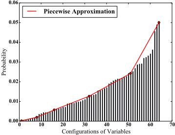
Our motivation for addressing the r-th order statistics problem is that a solution to it as well as a related problem of determining the rank of a given assignment will enable a number of interesting applications. First, it will enable us to get a deeper understanding of the underlying probability distribution (cf. [Ermon et al., 2013]). For example, by answering a linear number of order statistics queries, we can construct a piece-wise approximation of a complex probability distribution (see Figure 1). Such approximations can be useful for performing exploratory statistical analysis, understanding the shape of the distribution and visually comparing two probability distributions. Second, it will enable us to derive multiple, diverse explanations for evidence. Such explanations are extremely useful in interactive settings where users can provide feedback on the model and help correct its errors [Kulesza et al., 2015] (also see the recent DARPA Explainable AI program).
The r-th order statistic problem has received surprisingly little attention in the PGM literature. The problem has been shown to be P PP complete by reduction to Kth SAT [Kwisthout, 2008]. A closely related problem, that of enumerating all the m best solutions in a graphical model, has been investigated more thoroughly, with work extending back almost half a century [Lawler, 1972]. Work on the problem is ongoing; recent approaches include modifications of bestfirst search [Flerova et al., 2016] and formulation as a linear program [Fromer and Globerson, 2009].
The paper makes two contributions: (i) it theoretically analyzes the computational complexity of the r-th order statistics problem; and (ii) it introduces novel pseudo-polynomial time approximation algorithms for solving it. Specifically, we show that the r-th order statistics problem is NP-hard even when the graphical model has no edges (zero-treewidth or independent models). We prove this via a reduction from the number partitioning problem. Our reduction enables us to adapt pseudo-polynomial algorithms developed in the number partitioning literature for efficiently approximating the rth order statistics task in zero-treewidth models. To make this algorithm widely applicable, we extend it to general treedecompositions, which yields a practical algorithm for lowtreewidth graphical models. 1 The latter is non-trivial because unlike standard max and sum operators, arbitrary r-th order statistics operators such as the median are not associative.
We experimentally compared our new algorithm with a baseline sampling algorithm over randomly generated graphical models as well as Chow-Liu trees [Chow and Liu, 1968] computed over three benchmark datasets. We found that our new algorithm significantly outperforms the sampling algorithm, especially when r is not extreme (either too small or too large).
2 Preliminaries and Notation
Let X = {X1, . . . ,Xn} denote a set of n Boolean random variables, namely each variable Xi takes values from the set {0, 1}. We denote the assignments X1 = 1 and Xi = 0 by xi and xi respectively. Let Φ = {φ1, . . . , φm} denote a set of m non-negative real-valued functions (called potentials) where each φi is defined over a subset of variables of X called its scope and denoted by vars(φi). Then, the pair M = 〈X , Φ〉 is called a Markov network. M represents the following probability distribution:
where ω is a full (0/1) assignment to all variables in X, ωi is the projection of ω on vars(φi), and Z = ∑ω ∏mi=1 φi(ωi) is the partition function. We will denote the set of assignments to all variables in the set vars(φ) by Ω(vars(φ)). Often, we will abuse notation and denote Ω(X) by Ω. We will use ω to denote the assignment in which all variable assignments in ω are flipped. For example, if ω = (x1, x2, x3) then ω = (x1, x2, x3). For convenience, throughout the paper, we will assume Boolean variables noting that extension to multivalued variables is straightforward.
2.1 r-Order Statistics Query
Definition. Given a Markov network M〈X,Φ〉 and an assignment ω to all variables in X, the rank of ω is r, denoted by rankM(ω) = r, if there are exactly r assignments having lower or equal probability than ω in M. The r-order statistics query is to find an assignment having rank r in M.
A related query is finding the rank r given an assignment ω. We define the max (or min or median) assignment of a Markov network M〈X,Φ〉 as the assignment ω having the maximum (or minimum or median) rank. (For convenience, we always assume smaller of the two medians as the median.) The r-order statistics query is NP-hard in general because it includes the NP-hard most probable explanation (MPE) query of finding the max assignment as a special case.
1 In practice, if the treewidth of the graphical model is large, we can induce an accurate low-treewidth approximation of the model using variational inference methods such as mean field inference [Jordan et al., 1999] and Belief propagation [Yedidia et al., 2005].
3 Computational Complexity of r-Order Statistics on Independent Markov Networks
In this section, we analyze the computational complexity of computing order statistics on independent or zero-treewidth Markov networks, namely Markov networks, in which all potentials are univariate. Formally, ∀φ ∈ Φ, |vars(φ)| = 1. It is well known that max and the min assignments on such Markov networks can be computed in linear time. Surprisingly, as we show next, computing other order statistics, specifically finding the median assignment is intractable for these relatively simple models. Formally
Theorem 1. Given an independent Markov network M〈X , Φ〉, finding the median assignment ωmed is NP-hard.
Proof. Sketch. We reduce the optimization version of the number partition problem to the problem of computing the median assignment. Given a multiset S = {s1, . . . , sn} of positive integers, the number partitioning problem is to find a partition (S1, S2) of S such that | ∑g∈S1 g - ∑h∈S2 h| is minimized. Given S, we construct an independent Markov network M = 〈X , Φ〉 and show that given a median assignment to M, we can recover optimal (S1, S2) and vice versa.
M is constructed from S as follows. We have one Boolean variable Xi for each integer si in S. We have n univariate functions Φ = {φ1, . . . , φn} such that the scope of φi is {Xi} and
Our two claims, which we prove below are that (1) given an optimal partition (S1, S2) of S, the median assignment of M is the assignment having the smallest probability among the following two assignments: (a) the assignment obtained by setting all variables Xi such that si ∈ S1 to 1 and the remaining variables to 0, and (b) the assignment obtained by setting all variables Xi such that si ∈ S2 to 1 and the remaining variables to 0; and (2) given a median assignment ω to all variables of M, the optimal partition (S1, S2) of S is S1 = {si|xi ∈ ω} and S2 = {sj |xj ∈ ω}.
To prove our claims, we use the following two properties of independent Markov networks. First, we can re-parameterize each network so that there are exactly n univariate potentials, one for each variable, and each potential is normalized such that φi(xi) = 1 - φi(xi). For this re-parameterization, the partition function equals 1. For convenience, we will use the parameter pi to denote φi(xi). Thus, φi(xi) = 1 - pi. Second,
Proposition 1. Given an independent Markov network M there exists a constant µ such that ∀ω p(ω)p(ω) = µ.
The proof is straightforward:
We can use Proposition 1 to prove Lemma 1, thus proving the main claim in Theorem 1.
Lemma 1.
Proof. Without loss of generality, let us assume that ∑g∈S1 g ≤ ∑h∈S2 h, then Eq. (3) can be written as:
We will first prove that ωmed = argmaxω∈Ω≤ p(ω) where Ω≤ = {ω|p(ω) ≤ √µ}. Suppose that ∀ω1, ω2 ∈ Ω, p(ω1) ̸= p(ω2). Then |Ω≤| = 2n-1 , because for every pair (ω, ω), exactly one assignment is less than √µ and exactly one is greater than √µ. Therefore the median assignment must be the ω ∈ Ω≤ with the largest probability. In the general case, |Ω≤| ≥ 2n-1 , because for some pairs (ω, ω), its is possible that p(ω) = p(ω) = √µ. In this case, both ω ∈ Ω≤ and ω ∈ Ω≤. We can then partition Ω≤ into sets Ω< and Ω=, where |Ω<| < 2n-1 and |Ω<|+|Ω=| > 2n-1 . So, ωmed ∈ Ω=, and hence ωmed ∈ Ω≤ in this case as well.
Using Proposition 1, we can rewrite ωmed = argmaxω∈Ω≤ p(ω) as follows:
Next, we will simplify log(p(ω)) - log(p(ω)), which will make Eq. (7) equivalent to Eq. (4).
From Eq. (2), it is easy to see that log ( pi 1-pi ) = si. Thus, we can use Eq. (8) and Eq. (2) to rewrite Eq. (7) as:
Assigning all si such that xi ∈ ω to S1 and sj such that xj ∈ ω to S2 respectively, as described in Theorem 1, Eq. (9) is equivalent to Eq. (4) and the proof follows.
4 Estimating the Median in Independent Markov Networks
The relationship between the median finding problem in independent Markov networks and the partition problem gives insight into approaches we can use to compute order statistics. The good news is that the partition problem is "the easiest hard problem" [Hayes, 2002]; it is weakly NP-hard because it's time complexity is pseudo-polynomial, i.e. it is a polynomial function in the problem dimensionality and size of the integer inputs rather than the logarithm of the inputs.
Algorithm 1 Find Median Independent Markov Network
- 1: Input:A set of n probabilities {p1 . . . pn}, a precision, ϵ > 0.
- 2: Output: An estimate of the median assignment.
3:
- 4: function COMPUTEBIN(i, j)
5:
- if i < 0 ∨ j < 1 then return null
- 6: if i = 0 ∧ j = 0 then
- 7: b.c = 1
8:
for pi ∈ M do
9:
b.ω.Xi = xi
- 10: bfalse = COMPUTEBIN(i, j -1)
- 12: btrue.ω.Xi = xi
13: b.c = b.c + bfalse.c + btrue.c
- 14: b.ω = argmaxω∈b.ω,bfalse.ω,btrue.ω p(ω)
- 15: return b
16:
- 17: S = {}
- 18: for pi ∈M do
- 20: T = ⌈ ∑s∈S s 2 ⌉
- 21: while COMPUTEBIN(T, |S|).c = 0 do
- 22: T = T -1
- 23: return COMPUTEBIN(T, |S|).ω
The classical approach to solving the partition problem constructs a table with ⌊ ∑s∈S s 2 ⌋ rows and |S|+1 columns, in which cell bi,j tracks if there is an assignment to any subset of {s1 . . . sj} that sums to i. The algorithm populates each cell by a recurrence relation, whereby bi,j is true if and only if bi,j-1 is true (there is a subset of {s1 . . . sj-1} that sums to i), or bi-si,j-1 is true (there is a subset of {s1 . . . sj-1} that sums to i-si). Once constructed, the optimal solution can be retrieved by finding the largest row index for which the cell in the rightmost column is true.
For a Markov network M in which ∀φi ∈ Φ, log φi(xi) - log φi(xi) = si is integral, we can directly apply the dynamic programming approach to the multiset S = {s1 . . . sn} to find the exact value of the median. This condition will never be met in practice; in general we can quantize the difference log φi(xi) - log φi(xi) to obtain a median estimator with accuracy (and complexity) determined by the quantization size.
Algorithm 1 details our proposed approach. The algorithm accepts n parameters between 0.5 and 1, along with a precision ϵ (without loss of generality we assume that pi is the largest value in the normalized potential φi). For each pi, it computes a corresponding si by multiplying the quantity log pi - log(1 - pi) by ϵ and then rounding to the nearest integer. It computes an integer T as the ceiling of the sum of S divided by 2. Lines 4 - 15 define the recurrence relation. At each cell bi,j , we record two values; bi,j .c records the number of subsets of the first j variables that sum to i; bi,j.ω records the subset that corresponds to the maximum probability assignment. The algorithm computes the rightmost cell in descending row order until discovering a cell with a nonempty bin; it returns the maximal assignment in that bin as its estimate of ωmed.
5 Estimating arbitrary Ranks in Independent Markov Networks
Given an independent Markov network M, Algorithm 1 estimates the median by binning the assignments in the bottom half of Ω according to some quantization of their log-odds, and then returning the assignment with the largest probability in the largest bin. We can generalize this procedure in order to estimate the rank of any assignment in M by tracking more information in each bin; in addition to the max probability assignment, we modify Algorithm 1 to track the minimum probability assignment and the total number of assignments in each bin. We now run computeBin(i, |S|) for every value i ∈ [0 . . . ∑s∈S s] to retrieve a set of bins B representing a partition of the assignments of M, in which each b ∈ B contains b.c assignments ω such that p(b.min) ≤ p(ω) ≤ p(b.max). We refer to this data structure as a rank summary of M because it can be used to estimate the rank of any ω ∈ Ω.
Given a rank summary B and an assignment ω, we can partition B into 3 sets:
1. B< = {b ∈ B | p(b.max) < p(ω)} 2. B> = {b ∈ B | p(b.min) > p(ω)}- B= = {b ∈ B | p(b.min) ≤ p(ω) ≤ p(b.max)}
We know that ∑b∈B> b.c > rankM(ω) > ∑b∈B< b.c; however, for each b ∈ B=, we do not know how many of the b.c assignments have a smaller probability than ω. We can estimate this number by assuming the assignments in b are uniformly distributed between p(b.min) and p(b.max). Algorithm 2 details this proposed approach.
Algorithm 2 Estimate Rank
- 1: Input: A rank summary B computed using Algorithm 1 by tracking min, max and counts and an assignment ω ∈ Ω
- 2: Output: an estimate of rankM(ω)
- 3: r = 0
- 4: for b ∈ B do
- 5: if p(ω) > p(b.max) then
- 6: r = r + b.c
- 7: else if p(b.min) ≤ p(ω) ≤ p(b.max) then
- 8: r = r + p(ω)-p(b.min) p(b.max)-p(b.min) × b.c
- 9: return r
6 Rank Variable Elimination
Algorithms 1 and 2 describe a method for estimating the rank of assignments in independent Markov networks. In this section, we generalize this procedure to arbitrary Markov networks by combining it with the variable elimination algorithm for MPE inference [Dechter, 1999]. We describe the resulting algorithm, Rank Variable Elimination (RVE) next.
Variable elimination (VE) [Dechter, 1999] is a dynamic programming algorithm that accepts a Markov network M = 〈X,Φ〉 and an ordering O of X as input. For each X along the order O, VE: (1) discovers the set of potentials ΦX that mention X, (2) computes φX′ =⋊⋉φ∈ΦX φ, the join of the potential functions in ΦX (a product operation), (3) computes
Algorithm 3 Rank Variable Elimination
- 1: Input:A set of potential functions Φ with scope X, an ordering of X , O, a quantization function q(x)
- 2: Output: A rank summary of assignments ω ∈ Ω
- 3: Convert each potential φ in Φ to a rank potential ψ. Let Ψ denote the set of rank potentials
- 4: for each X along the order O do
- 5: ΨX = {ψ ∈ Ψ | X /∈ vars(ψ)}
- 6: ψ = ⋊ ⋉(ΨX );
- 7: ψ′ = ⊕(ψ,X);
- 8: Ψ = ΨX -ΨX ∪ {ψ′ };
- 9: return Ψ
φX = ⊕(φX′ ,X), the projection of the function φX′ onto φX with X removed from its scope (a max operation), and (4) updates the set of potentials by Φ = Φ - ΦX ∪ {φX}. When the algorithm terminates, Φ will contain a single potential with an empty scope and a single weight, which represents the MPE value of the input Markov network.
Algorithm 4 Rank VE ⋊⋉ Step
- 1: Input:A set of rank potentials Ψ 2: Output: A rank potential ψ 3: Y = ∪ψ∈Ψvars(ψ); ψ′ = {} 4: for ω ∈ Ω(Y) do 5: for ψi ∈ Ψ do 6: let 〈〈v1, b1〉 . . . 〈vm, bm〉〉 = ψi[ai] 7: v = v1 × . . . × vm 8: b.c = b1.c × . . . × bm.c 9: b.ωmin = b1.ωmin ∪ . . . ∪ bm.ωmin 10: b.ωmax = b1.ωmax ∪ . . . ∪ bm.ωmax 11: b.vmin = b1.vmin × . . . × bm.vmin 12: b.vmax = b1.vmax × . . . × bm.vmax 13: ψ′ [ω][v] = COMBINEBIN(b, ψ′ [ω][v]) 14: return ψ′
Algorithm 5 Rank VE ⊕ Step
- 1: Input:A rank potential ψ, an elimination variable X 2: Output: A rank potential ψ′ 3: ψ′ = {} 4: for 〈ω, v, b〉 ∈ ψ do 5: ω′ = ω -{X} 6: ψ′ [ω′ ][v] = COMBINEBIN(b, ψ′ [ω′ ][v])
- return ψ′
Each step of VE produces a simpler model by removing/maxing out one variable, thereby 'forgetting' information about weights that cannot be the max. The high-level idea behind Rank Variable Elimination (RVE) is to, at each step, group assignments with similar weights into a user-controlled number of bins via quantization, and then perform the max operation over each bin rather than over all possible assignments. Doing so lets us retain order statistics information that is traditionally discarded by VE.
In order to track this additional information, we define a new data structure, called a rank potential. A potential (function) is a map from all possible assignments to the variables in its scope to a non-negative real number; i.e.,
| Algorithm 6 Rank Variable Elimination Combine Bin Step | |
|---|---|
| 1: | Input:Two bins b1, b2 |
| 2: | Output: One bin b |
| 3: | b.c = b1.c + b2.c |
| 4: | if b1.vmin < b2.vmin or b2 = null then |
| 5: | b.ωmin = b1.ωmin; b.vmin = b1.vmin |
| 6: | else |
| 7: | b.ωmin = b2.ωmin; b.vmin = b2.vmin |
| 8: | if b1.vmax > b2.vmax or b2 = null then |
| 9: | b.ωmax = b1.ωmax; b.vmax = b1.vmax |
| 10: | else |
| 11: | b.ωmax = b2.ωmax; b.vmax = b2.vmax |
| 12: | return b |
φ = {〈ω1, v1〉 . . . 〈ωn, vn〉} where ωi ∈ Ω(vars(φ)), vi ∈ R+ ∪ {0}, and n = 2|vars(φ)| . In a rank potential, we replace each vi with a function, called a binning function. A binning function maps from integral-valued 'quantizations' of the intermediate weights generated during VE to a data structure we call a bin, which tracks information needed to estimate order statistics throughout RVE. We define this data structure next.
Definition. A quantization function q(x) : R+ ∪ {0} → Z is a function such that ∀x, y ∈ R, q(x)q(y) ≈ q(xy).
Definition. A binning function b(x) : Z → B is a function that maps from the integers to the set of bins, B = {〈ωmin, ωmax, vmin, vmax, c〉 | ωmin, ωmax ∈ Y, Y ⊆ X , vmin, vmax ∈ R+∪{0}, c ∈ N}
Definition. A rank potential is a set of pairs ψ =
{〈ω1, b1(z)〉. . .〈ωn, bn(z)〉}, where ωi ∈ Ω(vars(ψ)) and each bi is a function bi(z) : Z→B.
Algorithm 3 describes the steps in RVE. Given a set of potentials, an ordering, and a quantization function, line 3 constructs one rank potential ψ from each potential φ in the Markov network. Specifically, for each potential value (ω, v) in φ, we construct a bin by setting its min and max values of to v, its min and max assignments to ω, and the count to 1. Lines 9 - 11 of Algorithm 3 mirror traditional VE. The difference is that the product (⋊⋉) and project (⊕) operators are defined over rank potentials. We describe these operators next.
Product Operator. Algorithm 4 describes the product operation for rank potentials. It first computes Y, the union of the scopes of all input rank potentials, Ψ. For each possible assignment ω to all variables in Y, it retrieves {ψ1[ω], . . . ψm[ω]}, the binning function from each ψ ∈ Ψ consistent with ω. Next, it computes a new binning function, ψ′ [ω], by taking the cartesian product of they key-value pairs in {ψ1[ω], . . . ψm[ω]}. Each created bin requires updating 5 values; assignments are computed as union of the assignments of each bin in the product (assignments are guaranteed to be consistent over shared variables), values are updated as products of values (as in the product step of VE), and counts are updated as the product of counts. Algorithm 4 computes the new bin key v as the product of bin keys; because q(x)q(y) ≈ q(xy), we expect this value to be approximately the quantization of all assignments in our newly created bin. Line 13 inserts the new bin to the binning function for ψ′ [ω] under quantized key v (after checking for collisions, discussed below). Once completed for all assignments
ω, the algorithm returns ψ′ .
Project Operator. Algorithm 5 describes the project operation for rank potentials. For each triple 〈ω, v, b〉 ∈ ψ, where ω ∈ Ω(vars(ψ)), v ∈ Z, and b ∈ B, it 'forgets' the assignment to elimination variable X by creating a new assignment ω′ = ω - {X}, and adding b to the new rank potential ψ′ under assignment ω′ with binning key v (after checking for collisions). Once done for all triples, the returns new rank potential ψ′ , where vars(ψ′ ) = vars(ψ) - {X}.
When creating new rank potentials, Algorithms 4 and 5 must check for bin collisions. Bin collisions occur when two different bins quantize to the same binning key. Algorithm 6 describes the combine operation for colliding bins. Again, 5 values must be updated. The max and min values of the combined bin become the max of the max values and the min of the min values, respectively. The max and min assignments become the assignments corresponding to the max of the max values and the min of the min values, respectively. Finally, the count of the combined becomes the sum of the counts of the colliding bins.
Upon completion, Algorithm 3 returns Ψ = {ψ}, where ψ = {〈{}, q(x)〉}, i.e. it returns a single binning function, q(x) : Z → B. Every assignment to X has been placed in some bin in B, i.e. ∑b∈B b.count = 2|X| . Given an arbitrary assignment, the rank of that assignment can be estimated by the same process described in Algorithm 2.
Analysis of Algorithms 3, 5, 4, and 6 yields the following:
Theorem 2. Given a Markov network M having n variables, an ordering O having width w, and a quantization function that generates a maximum of k bins at every elimination step, the time and space complexity of Algorithm 3 is O(n × k × exp(w)).
7 Experimental Results
In this section, we aim to evaluate the performance of Algorithms 1 and 3. We use the RVE algorithm to estimate solutions to two types of queries: (1) Infer Rank given an assignment. and (2) Infer the assignment given a rank. To solve the latter query using RVE we apply Algorithm 2 to the min and max tuple stored in each bin, and return the assignment whose rank estimate ˆ r minimizes |r - ˆ r|.
Because of the lack of established approximation algorithms for the order statistics query, we use the following straightforward sampling-based approach as a baseline. We first sample a multiset T of assignments from the uniform distribution. Given a Markov network M having n variables and an assignment ω, let lT be the number of samples that have smaller (or equal) probability than ω according to M, then our estimate of the rank of ω is lT |T| 2n . Similarly, the estimate of the assignment having rank r is the assignment having rank ⌊ r 2n |T |⌋ in T .
7.1 Inferring Rank of an Assignment
We evaluate the infer rank query on 3 benchmark datasets commonly used for evaluating learning algorithms for tractable probabilistic models: NLTCS, KDD Cup, and Plants [Lowd and Davis, 2010; Rahman and Gogate, 2016; Gens and Domingos, 2013]. We first learn a Chow-Liu tree for each dataset. For each model, we generate 1000 random assignments to all variables. For each assignment, we run RVE on the corresponding model to estimate its rank and record the time taken to compute the estimate. We give the sampling algorithm the same amount of time to compute an estimate.
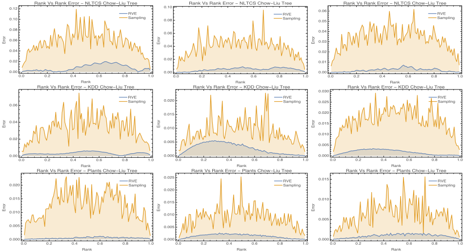
For NLTCS (16 variables), we find the true rank of each assignment by computing the probability of all complete assignments and sorting them. For the KDD Cup and Plants datasets (with 64 variables and 69 variables, respectively), we estimate the true rank of each assignment by running the sampling algorithm for 600 seconds. We compute rank error for each assignment as |ˆ r-r| 2n , where n is the number of variables in the model. We use quantization function q(x, α) = ⌊α log x⌋, and run the experiment for varying settings of α. For each model and α, we plot the error in rank as a function of the normalized true rank of the assignment. From the set of 1000 random samples, we generate 100 data points by rounding each true rank to its nearest percentile value and averaging the errors.
Figure 2 shows the results. We observe that sampling tends to perform well towards the extreme values of the distribution, but struggles to accurately predict rank for assignments near the middle of the distribution. Its accuracy appears to depend only on time and number of variables in the model. RVE outperforms sampling by a significant margin in all tested distributions for all choices of α. The variance in its accuracy (as a function of true rank) appears to be distribution dependent; for example, on the NLTCS dataset, increasing α improves the overall accuracy of the algorithm, but its highest error remains in the same range of ranks in each case (normalized ranks in [0.5, 0.8]). In general, RVE will perform the worst in the ranges of the distribution that are most densely populated because the bins corresponding to these locations will contain more assignments. Dynamic binning strategies might be effective in such cases and we leave this for future work.
7.2 Inferring Assignment having a given Rank
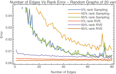
We evaluate infer assignment at rank queries on synthetic models generated by the following procedure. For each e ∈ [0, 80], we generate 100 Markov networks on 20 variables with e pairwise potentials having randomly generated scopes. The weights of each potential are randomly generated from N (0, 1). For each Markov network, we use RVE to estimate the the tuple at normalized rank [0.05, 0.50, 0.95%]. We then run the sampling algorithm for the same queries for the same amount of time. We calculate the true rank of the assignments returned by each algorithm, and report the error.
Figure 3 shows the results. We observe that RVE outperforms sampling by a significant margin for sparse models, but that sampling becomes more viable as we increase the number of edges. Because RVE is a VE-based algorithm, its complexity is exponential in treewidth, whereas the accuracy of the sampling algorithm is determined only by the number of variables in the model and the number of samples generated. Thus, the sampling approach becomes more viable the more densely connected the models become. For randomly generated models, both algorithms perform better when searching for assignments at the extremes of the distribution; however, the sampling approach has higher variance than RVE when its accuracy is viewed as a function of the rank.
8 Conclusion
In this work, we have introduced a new query type for the graphical model domain, namely, computing the order statistics of a PGM. We have shown that the task is NP-hard even for zero-treewidth models. To our knowledge, we have presented the first deterministic algorithm for estimating the order statistics problem by combining a well-known approach to solving the Partition Problem with the standard variable elimination algorithm for PGMs. We have demonstrated that our approach can return better results than sampling on a number of synthetic and real-world problems.
Acknowledgements
This research was funded in part by the DARPA Probabilistic Programming for Advanced Machine Learning Program (contract number FA8750-14-C-0005), DARPA Explainable Artificial Intelligence Program (contract number N66001-172-4032) and by the NSF awards 1528037 and 1652835. The views and conclusions contained in this document are those of the authors and should not be interpreted as representing the official policies, either expressed or implied, of DARPA, NSF or the US government.
@inproceedings{ijcai2017p645,
  title     = {Order Statistics for Probabilistic Graphical Models},
  author    = {Smith, David and Rouhani, Sara and Gogate, Vibhav},
  booktitle = {Proceedings of the Twenty-Sixth International Joint Conference on
               Artificial Intelligence, {IJCAI-17}},
  publisher = {International Joint Conferences on Artificial Intelligence Organization},
  editor    = {Carles Sierra},
  pages     = {4625--4631},
  year      = {2017},
  month     = {8},
  note      = {Main track},
  doi       = {10.24963/ijcai.2017/645},
  url       = {https://doi.org/10.24963/ijcai.2017/645},
}
TY - CPAPER TI - Order Statistics for Probabilistic Graphical Models AU - Smith, David AU - Rouhani, Sara AU - Gogate, Vibhav T2 - Proceedings of the Twenty-Sixth International Joint Conference on Artificial Intelligence, IJCAI-17 PB - International Joint Conferences on Artificial Intelligence Organization PY - 2017 SP - 4625 EP - 4631 DO - 10.24963/ijcai.2017/645 UR - https://doi.org/10.24963/ijcai.2017/645 ER -Copied
Machine-readable versions of this paper, for tools and AI agents:





