
Variational Mixtures of Gaussian Processes for Classification
Proceedings of the Twenty-Sixth International Joint Conference on Artificial Intelligence. Main track. Pages 4603-4609.
https://doi.org/10.24963/ijcai.2017/642
Keywords
- Uncertainty in AI: Approximate Probabilistic Inference
- Uncertainty in AI: Graphical Models
Abstract
Gaussian Processes (GPs) are powerful tools for machine learning which have been applied to both classification and regression. The mixture models of GPs were later proposed to further improve GPs for data modeling. However, these models are formulated for regression problems. In this work, we propose a new Mixture of Gaussian Processes for Classification (MGPC). Instead of the Gaussian likelihood for regression, MGPC employs the logistic function as likelihood to obtain the class probabilities, which is suitable for classification problems. The posterior distribution of latent variables is approximated through variational inference. The hyperparameters are optimized through the variational EM method and a greedy algorithm. Experiments are performed on multiple real-world datasets which show improvements over five widely used methods on predictive performance. The results also indicate that for classification MGPC is significantly better than the regression model with mixtures of GPs, different from the existing consensus that their single model counterparts are comparable.
- [Bishop and Svenskn, 2003] Christopher M. Bishop and Markus Svenskn. Bayesian hierarchical mixtures of ex- perts. In Proceedings of the 19th Conference on Uncer- tainty in Artificial Intelligence, pages 57-64, 2003.
- [Bishop, 2006] Christopher M. Bishop. Pattern Recognition and Machine Learning. Springer, 2006.
- [Blei and Jordan, 2006] David M. Blei and Michael I. Jor- dan. Variational inference for Dirichlet process mixtures. Bayesian Analysis, 1:121-144, 2006.
- [Blei et al., 2016] David M. Blei, Alp Kucukelbir, and Jon D. McAuliffe. Variational inference: A review for statisticians. ArXiv e-prints:1601.00670, 2016.
- [Ferguson, 1973] Thomas S. Ferguson. A Bayesian analysis of some nonparametric problems. The Annals of Statistics, 1:209-230, 1973.
- [Gal et al., 2015] Yarin Gal, Yutian Chen, and Zoubin Ghahramani. Latent Gaussian processes for distribution estimation of multivariate categorical data. In Proceed- ings of the 32nd International Conference on International Conference on Machine Learning, pages 645-654, 2015.
- [Hensman et al., 2015] James Hensman, Alexander G. de G. Matthews, and Zoubin Ghahramani. Scalable variational Gaussian process classification. In Proceedings of the 18th International Conference on Artificial Intelligence and Statistics, pages 351-360, 2015.
- [Kapoor et al., 2010] Ashish Kapoor, Kristen Grauman, Raquel Urtasun, and Trevor Darrell. Gaussian processes for object categorization. International Journal of Com- puter Vision, 88:169-188, 2010.
- [Lichman, 2013] M. Lichman. UCI machine learning repos- itory, 2013.
- [Meeds and Osindero, 2006] Edward Meeds and Simon Osindero. An alternative infinite mixture of Gaussian pro- cess experts. Advances in Neural Information Processing Systems, 18:883-890, 2006.
- [Rasmussen and Ghahramani, 2002] Carl Edward Ras- mussen and Zoubin Ghahramani. Infinite mixtures of Gaussian process experts. Advances in Neural Information Processing Systems, 14:881-888, 2002.
- [Rasmussen and Williams, 2006] Carl Edward Rasmussen and Christopher K. I. Williams. Gaussian Processes for Machine Learning. The MIT Press, 2006.
- [Sethuraman, 1994] Jayaram Sethuraman. A constructive definition of Dirichlet priors. Statistica Sinica, 4:639-650, 1994.
- [Smola and Bartlett, 2001] Alex J. Smola and Peter L. Bartlett. Sparse greedy Gaussian process regression. Advances in Neural Information Processing Systems, 13:619-625, 2001.
- [Sun and Xu, 2011] Shiliang Sun and Xin Xu. Variational inference for infinite mixtures of Gaussian processes with applications to traffic flow prediction. IEEE Transactions on Intelligent Transportation Systems, 12:466-475, 2011.
- [Tresp, 2001] Volker Tresp. Mixtures of Gaussian pro- cess. Advances in Neural Information Processing Systems, 13:654-660, 2001.
- [Yuan and Neubauer, 2009] Chao Yuan and Claus Neubauer. Variational mixture of Gaussian process experts. Advances in Neural Information Processing Systems, 21:1897-1904, 2009.
References were extracted automatically from the PDF and may contain errors.
Full text extracted automatically from the PDF; figures, tables and equations may differ. The PDF is the version of record.
1 Introduction
Gaussian Processes (GPs) specify a collection of latent random variables f which have a joint Gaussian distribution [Rasmussen and Williams, 2006]. GP is a powerful tool for probability modeling in machine learning and has been applied to both classification and regression problems with different kinds of likelihood p(y|f ) where variables y are outputs. Gaussian likelihood is the typical choice for regression models, which leads to convenience in derivation. Logistic and probit functions are commonly used in GP classification models where inferences are not in closed form. In general, both GP regression and classification models are discriminative models, i.e., only the conditional distribution p(f|X) is formulated.
GP-based mixture models have been proposed for overcoming the limitations of single GP models: First, GP is incapable of handling multi-modality in data. Second, the computational complexity for calculating the inverse kernel matrix is O(N 3 ) with N being the number of training points. Tresp [2001] proposed the mixture of GP regression models with finite mixture components. Rasmussen and Ghahramani [2002] introduced a Dirichlet Process (DP) based gating network and extended the mixture of GPs to accommodate an infinite number of components. The first limitation is overcome by incorporating multiple GPs. The cubic computational complexity is resolved through replacing the inversion of a large kernel matrix by inversions of multiple small matrices. For each component, only a subset of training set is used for calculating the kernel matrix, which leads to lower computational complexity. InMeeds and Osindero [2006], inputs are assumed to be Gaussian distributed. The distribution of inputs is involved in gating network for effective estimations of mixture weights. This modification adapts previous discriminative models to generative ones. Markov Chain Monte Carlo (MCMC) methods are adopted for approximate posterior inference in the above work. However, MCMC methods demand expensive time for both training and prediction. The convergence of these methods is also difficult to identify.
Variational inference is a deterministic approximate technique which is a commonly used alternative for MCMC methods [Bishop, 2006]. The idea of variational inference is approximating intractable true posterior distribution p(z|X) with a variational distribution q(z) by minimizing the KL divergence between q(z) and p(z|X). It presents an analytical formulation of approximate posterior distribution, which simplifies the integrals in model training and prediction.
A finite mixture model of GP experts which employs variational inference has been proposed in [Yuan and Neubauer, 2009]. Recently, Sun and Xu [2011] proposed a new variational approximation algorithm for the infinite mixture model of GPs and applied it to traffic prediction problems. In the above work, the variational distribution of latent variables is assumed to have a fully factorized form, i.e., latent variables are independent of each other. Thus, the expectations taken with respect to q(z) are decoupled, which simplifies calculations greatly. Following this assumption, the technique is known as mean field variational inference. Although with simple posterior assumptions, mean field variational inference is a good choice for approximate posterior inference [Blei et al., 2016] and commonly used in recent work [Gal et al., 2015; Hensman et al., 2015].
All of the previous work about mixtures of GPs only focuses on regression problems, i.e., the Gaussian likelihood is employed. Inspired by the GP classification model and mixtures of GPs, we propose a generative Mixture of Gaussian Processes for Classification (MGPC) which extends mixtures of GP regression models to a classification model. Similar with Sun and Xu [2011], a linear GP model is employed. The linear GP model is equivalent to GPs and breaks the dependencies among outputs. This property enables mean field variational inference for mixtures of GPs feasible. We validate our model on multiple binary classification datasets. Because binary classification problems can be regard as restricted regression problems whose outputs only take values in {-1,+1}. The mentioned regression models, including the GP regression model and mixture model of GPs, are also amenable for classification. The signs of outputs of such models are used for making predictions. The experiments are performed with both classification and regression models for comprehensive comparisons.
The rest of this paper is organized as follows. Section 2 introduces our model with a brief overview of necessary background. Then, Section 3 gives the details of variational inference and optimization algorithms. In Section 4, we present classification performances on real-world datasets and provide interesting discussions. Finally, we give conclusion in Section 5.
2 The ProposedModel
The GP jointly models outputs as a multivariate Gaussian distribution. The linear GP model is an equivalent parametric representation to the GP, which introduces an intermediate variable for breaking the dependencies among outputs. The conditional independencies not only facilitate derivations of variational inference but also simplify the predictive distribution, which we will show in Section 3. In this section, we first introduce the GP and linear GP model with their equivalence. Then we give a brief introduction about the stick-breaking construction of DPs. Finally, we show the graphical representation and details of our model.
2.1 Gaussian Processes
A noise-free GP f is specified as
where κ(·, ·) is the kernel function (a.k.a., covariance function). For inputs X = {xn}Nn=1 , the joint distribution of outputs is given by a multivariate Gaussian distribution,
where Kxx is the N × N kernel matrix obtained by κ(·, ·). We can see that the dependencies among f are specified by Kxx implicitly.
Now we introduce the intermediate variable w to formulate the linear GP model. Variable w is Gaussian distributed as N (0, K-1 xx ). The linear GP model is specified by a univariate Gaussian distribution as follows,
where r is the inverse variance and φ(x) is a vector defined by covariance function
Actually, Kxx = [φ(x1), φ(x2), ...φ(xN)]. We recover f = [f1, f2, ...fN]⊤ through f = Kxxw + ξ where ξ has a Gaussian distribution N(0, r-1 ). It shows that f has a multivarate Gaussian distribution N(0,Kxx + r-1E) which is equivalent to GP with independent noise N(0, r-1E), where E is the identity matrix. Further, given {x,w, r}, the outputs are conditional independent.
Now, we introduce the mixture of GPs. Each component in our model has the formulation of Eq. (3) with different parameters and is assumed to have a support set It of M training instances, which is a subset of the complete training set. z is a variable which indicates the corresponding component that the instance belongs to. Given z = t, f is distributed as N (w⊤ t φt(x), r-1 t ). φt(x) andKt are calculated over support set It through covariance function κt(·, ·). Variable wt has a Gaussian distribution N(0,U-1 t ) where Ut = Kt + σ2 tbE. The additional termσ2 tbE aims to avoiding matrix singularity. We assume that rr has a gamma distribution Γ(rt|a0, b0).
We choose the radial basis function kernel with automatic relevance determination [Rasmussen and Williams, 2006] for each component, whose formulation is
where Λ = diag(σ2 t1 , σ2 t2 , ..., σ2 td ) with d denoting the dimension of x. The hypermeters that define the kth GP component are covariance function parameter θt = {σtb, σtf , σt1, σt2, ..., σtd} and support set It.
2.2 Dirichlet Processes
The DP [Ferguson, 1973] is a commonly used prior model for Bayesian nonparametric modeling. A draw from a DP is a discrete distribution over countably infinite atoms. Thus, the DPs have been adopted to extend finite mixture models to accommodate countably infinite components, where each atom represents a mixture component. The stick-breaking construction of DPs [Sethuraman, 1994] is adopted for our model.
Suppose that H is a base distribution. Φ = {Φ1,Φ2, ...,Φ∞} and ν = {ν1, ν2, ..., ν∞} are two infinite sets of independent random variables which are drawn from H and Beta(1, α0), respectively. Correspondingly, infinite proportion variables π = {π1, π2, ..., π∞} are introduced for representing the probabilities for atoms in Φ. For the kth atom, πi = νi ∏i-1 j=1 (1 - νj). The stick-breaking construction of the DP G is formulated as
where δΦi is the delta function at Φi. This construction is analogous to breaking a stick with unit length for infinite times. First, we break the stick into two parts at position ν1, i.e., π1. The stick of length-π1 is the current stick and the rest is the remaining stick which has length-(1 - ν1). Then we repeat breaking the remaining stick, infinitely. Clearly, ∑∞i=1 πi = 1, and G is a discrete distribution.
The distribution of component indicator variable z is regarded as a categorical distribution Cat(π). More formally, given ν, the distribution p(z|ν) is
where 1[z > t] and 1[z = t] are indicator functions.
2.3 Mixtures of Gaussian Processes for Classification
In this section, we will introduce the details of MGPC. First, suppose that training set D is {(xn, yn)}Nn=1 . The complete latent variable set is Ω = {ν,µ,R,w, r, z, f}, where ν = {ν1, ν2, ..., ν∞}, µ = {µ1,µ2, ...,µ∞}, R = {R1,R2, ...,R∞}, w = {w1,w2, ...,w∞}, r = {r1, r2, ..., r∞}, z = {z1, z2, ..., zN}, and f = {f1, f2, ..., fN}. The complete hyperparameter set Θ is {θ, I, α0, µ0, R0,W0, ν0, a0, b0}, where θ = {θ1, ..., θ∞} and I = {I1, ..., I∞}. In the following, we will explain the details of these terms.
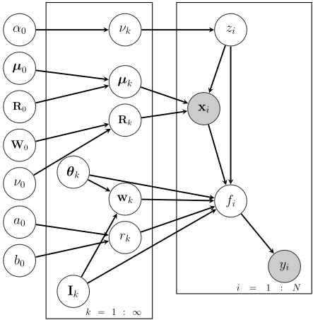
Figure 1 shows the graphical representation of MGPC. We demonstrate the model in a top-down order. For clarity, the indices of inputs and outputs are omitted. We use +1/ - 1 labels for output y. Given f, the probability p(y = +1|f) = σ(f) where σ(·) is the logistic function. As the symmetry of the logistic function, the above probability can be written as p(y|f) = σ(yf). The latent variable f is given by the mixture of GPs and σ(·) is deterministic. Therefore, y also has multi-modality. For the kth component, we have a Gaussian distribution N(w⊤ k φk(x), r-1 k ), i.e., a linear GP model as described previously. Given the mixture component k, the input x is Gaussian distributed where µk and Rk are corresponding mean and inverse covariance, respectively. Further, µk is Gaussian distributed N(µ0,R-1 0 ), and Rk is Wishart distributedW(W0, ν0). z is the latent variable that indicates the component assignment for instance {x, y}.
The joint distribution of our model is
where xn and fn obey the mixture of Gaussian distributions and mixture of GPs, respectively,
k = 1 : ∞
Figure 1: Graphical model representation of MGPC.
Note that xn and fn share the infinite components. Thus, given an input x, the mixture weight of the kth component is dependent on x, which is given by
The details of the inference and optimization of our model will be introduced in the next section.
3 Variational Inference and Optimization Algorithms
The posterior distribution p(Ω|D) is not in closed form because ∫ p(Ω,D)dΩ is intractable. So we resort to mean field variational inference to approximate p(Ω|D).
For general latent variables z and observation X, the objective function, i.e., the lower bound, is given by
With the mean field assumption of variational distributions, the optimization algorithm for maximizing the lower bound is an iterative procedure. Each factor is updated in turn while fixing the others, which is known as the coordinate ascent algorithm. For the ith latent variable zi, the solution is
In our model, the solutions of updating q(ν), q(µ), q(R), q(w), q(r) and q(z) are in closed form. For q(f), we adopt a gradient-based method to optimize it by maximizing the lower bound. A specific form of q(f) is required . Then the parameters are updated according to their gradients.
All of the hyperparameters except θ in the covariance function and support set I are fixed because such hyperparameters are generic without the need for further estimation. We set such hyperparameters following [Bishop and Svenskn, 2003; Blei and Jordan, 2006; Yuan and Neubauer, 2009; Sun and Xu, 2011]. The variational EM algorithm is employed for learning θ where the expectation is calculated over variational distribution and a greedy algorithm is used to update support set I.
3.1 Variational Inference
Following the fully factorization assumption and truncated stick-breaking representation of DPs, the variational distribution is formulated as
where T is the truncation level of the DP.
When optimizing variational distribution according to Eq. (13), all of the solutions are in closed form except q(f) [Blei et al., 2016]. The derivations of variational distributions in closed form is standard and analogous to the Gaussian likelihood situation [Yuan and Neubauer, 2009; Sun and Xu, 2011]. Thus, the details of such solutions are omitted in this paper.
Now, we present the details of updating q(fn). Each fn is given by a mixture of Gaussian distributions and output yn is generated by the weighted average of T components. We assume that q(fn) has a Gaussian distribution N(µn, σn), i.e., a best single Gaussian distribution is desired for approximating the original mixture of Gaussian distributions. Substituting the Gaussian probability density function into Eq. (12) and absorbing independent terms into the constant, we obtain the following objective function,
However, the second integral, namely, Eq(fn) lnp(yn|fn), is not in closed form. A Monte Carlo-based approximate method [Gal et al., 2015] has been proposed to handle such situation with the cost of sampling. Instead, we optimize a lower bound of such integral which is obtained by E ln [1+ e-ynfn ] ⩽ lnE [1+ e-ynfn ]. The first integral is analytical and the last one is the entropy of the Gaussian distribution. Thus, the surrogate objective function is formulated as follows,
All the expectations are calculated with respect to the variational distribution. The derivatives of parameters are provided below,
With the gradients of the parameters, the conjugate gradient method is employed for maximizing the surrogate objective function given by Eq. (16).
3.2 Optimization for Hyperparameters
Let ˆΘ = {θ1:T , I1:T} be the hyperparameters to be optimized. The other hyperparameters are fixed to generic values. For covariance function variables θ, we adopt the variational EM algorithm to maximize Eq(Ω) ln p(D, Ω|θ). For support sets I, we follow the method in [Smola and Bartlett, 2001; Yuan and Neubauer, 2009; Sun and Xu, 2011].
When optimizing θ, the objective function is
where the irrelevant terms to θ are omitted. Suppose the variational distributions of wt and fn are N(µ,Σ) and N(µn, σn), respectively. Substituting the corresponding probability density functions and calculating the expectations, the objective function with respect to each θk is simplified as
where A = (Σ+µµ⊤), b = Ert. Then we maximize the objective function through the conjugate gradient method. The derivation of gradients are omitted.
The support sets I are optimized by a greedy algorithm [Smola and Bartlett, 2001; Yuan and Neubauer, 2009]. For each support set It, the objective is the density of q(wt) at its mean. As wt has a Gaussian distribution, the above objective is equivalent to maximizing the determinant of the inverse covariance matrix. The instances are greedily selected for maximizing the objective from candidate sets which are randomly sampled from the training set.
Now, we introduce the whole procedure of model training. First, the hyperparameters ˆΘ are initialized. The support sets are initialized by the K-means algorithm which clusters the training set into T components. Then variational inference is run to obtain the approximate posterior distribution q(Ω). The variational EM algorithm is performed to update θ. Fixing θ and variational distributions except q(w), each support set It is filled by the greedy algorithm in turn. Based on the updated support sets, the above steps are repeated until the variations of the support sets are under a predefined threshold or the maximum iteration number is reached.
3.3 Predictive Distribution
The predictive distribution for a new input x∗ is given by
Approximations are necessary for computations of both p(f ∗ |x∗ ,D,Ω,Θ) and the integral. For p(f ∗ |x∗ ,D,Ω,Θ), we approximate it as follows,
where the true posterior distribution is approximated by the variational distribution and then posterior means ˆΩ are further employed. As the parametric representation of GPs, we have the conditional independence property of the outputs f . Thus the predictive distribution is simplified as,
Because the integral in Eq. (23) is intractable, we adopt the approximate method from [Bishop, 2006] as
The mixture weight p(z∗ = t|x∗ , ˆΩ) is calculated as in Eq. (11) with posterior means of the variational distribution.
4 Experiments
In this section, we evaluate our proposed model MGPC on multiple real-world datasets and compare it with existing classification models including Gaussian Process Classification models (GPC), SVM and Logistic Regression (LR). As mentioned in Section 1, regression models can also perform binary classification. We evaluate classification performances of Gaussian Process Regression models (GPR) and Mixtures of Gaussian Processes for Regression (MGPR) [Sun and Xu, 2011]. We report the experimental results with corresponding analyses from three viewpoints: comparisons of classification performances, classification versus regression models, and mixture versus single models.
| Dataset | # of instances | # of features |
|---|---|---|
| Blood | 748 | 3 |
| Fertility | 100 | 9 |
| Haberman | 306 | 3 |
| Housevotes | 435 | 16 |
| Mammographic | 830 | 5 |
| Parkinsons | 195 | 22 |
| Pima | 768 | 8 |
| Heart | 270 | 13 |
| Iris | 150 | 4 |
4.1 Datasets and Setups
Table 1 shows the information about the used datasets. All of the datasets are available on UCI data repository [Lichman, 2013]. The iris dataset has 3 classes in total. We perform experiment on the instances of label "Versicolour" and "Virginica" because the classification accuracies are consistently 100% on other combinations for each model.
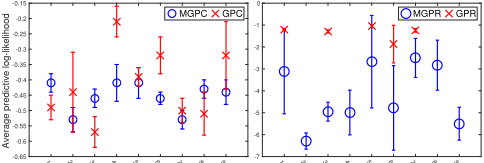
All of the datasets are randomly split into the training, validation and test set by a ratio of 4:3:3. The truncation level T and the initializations for variance parameters of q(fn) are selected using the validation set. T is set to range from 2 to 4, and the corresponding size of the support set for each component is set to Ntrain/T. The variance σn are initially set to range in 0.005 × [1, 2, 4, 8, 16, 32]. We run experiments on randomly split datasets for 10 times and report the average accuracies in percentage with corresponding standard deviations in Table 2. The comparisons of predictive log likelihoods of MGPC, MGPR, GPC and GPR on the test sets are also provided in Figure 2.
4.2 Classification Performances
From Table 2, we can see that MGPC outperforms all of the other models on 7/9 datasets. For the rest of the datasets, GPC and GPR obtain the best performance, respectively. We also run paired t-test on average accuracies over all datasets for further comparisons of MGPC and other models. The results are reported in Table 3. As we can see, all of the p-values are less than 5%, which indicates the significant improvements of MGPC.
4.3 Classification versus RegressionModels
For binary classification, regression models are also amenable. Empirical results show that the classification performances of GPC and GPR are typically comparable [Kapoor et al., 2010]. For further evaluating performance differences between classification and regression models, we evaluate regression models including MGPR and GPR and compare the performances with MGPC and GPC, respectively. The classification accuracies have been shown in Table 2 as well as the average predictive log likelihoods with standard deviations in Figure 2. For clarifying the performance differences between classification and regression models, paired t-test results are indicated for each datasets with arrows, respectively.
| Dataset | Mixture Model | Single Model | ||||
|---|---|---|---|---|---|---|
| MGPC | MGPR | GPC | GPR | SVM | LR | |
| Blood | 78.50±2.53(0.4681) | 77.63 ±2.49 | 77.92 ±3.36 | 77.79 ±3.55 | 77.78 ±2.43 | 77.74 ±3.25 |
| Fertility | 88.00±4.83(0.0575) | 84.67 ±5.26 | 85.67 ±4.98 | 85.33 ±5.49 | 86.67 ±4.71 | 80.33 ±6.56 |
| Haberman | 75.41±4.67(0.1724) | 73.68 ±3.04 | 72.80 ±2.88 | 72.13 ±2.23 | 73.13 ±2.48 | 72.68 ±2.34 |
| Housevotes | 95.33±1.96(0.0386) | 93.27 ±3.97 | 94.48 ±2.37 | 94.33 ±2.28 | 95.10 ±2.27 | 94.33 ±1.83 |
| Mammographic | 83.49 ±2.31(0.6380) | 83.21 ±1.81 | 84.02 ±2.62 | 84.62±2.26 | 81.57 ±1.91 | 82.37 ±2.51 |
| Parkinsons | 87.56±2.49(0.0276) | 82.92 ±4.17 | 86.59 ±5.38 | 83.34 ±5.79 | 85.89 ±5.27 | 75.23 ±8.43 |
| Pima | 76.91±3.34(0.0014) | 73.57 ±1.45 | 75.28 ±3.18 | 74.80 ±3.47 | 76.33 ±2.15 | 76.11 ±1.67 |
| Heart | 80.62 ±3.19(0.0437) | 76.05 ±5.15 | 80.74±4.20 | 78.77 ±4.50 | 80.59 ±3.79 | 75.56 ±5.91 |
| Iris | 96.00±3.06(0.3938) | 95.00 ±2.83 | 93.67 ±4.29 | 92.33 ±3.53 | 94.67 ±4.77 | 94.33 ±3.87 |
| MGPR | GPC | GPR | SVM | LR | |
|---|---|---|---|---|---|
| MGPC | 0.0020 | 0.0132 | 0.0063 | 0.0026 | 0.0247 |
1
2
3
4
5
6
7
8
9
1
2
3
4
5
6
7
8
9
Figure 2: Average predictive log likelihoods. The average predictive log-likelihoods with deviations are plotted in the same order as Tabel 1. For clarity, the names of the datasets are omitted. In the right figure, four points which have extremely small values are omitted for GPR.
As shown in Table 2, the performances of GPC and GPR are not significantly different, which is in accordance with previous empirical consensus. However, this phenomenon is not preserved for MGPC and MGPR. Significant improvements are obtained by MGPC on 4/9 datasets.
Additionally, as shown in Figure 2, the predictive log likelihoods for classification models are much larger than that for regression models. The regression models make predictions according to the signs of outputs and do not evaluate probabilities of predicted labels directly, which leads to inferior estimations of the distribution of the test data. When the predictive distributions are highly aggregated at wrong labels (i.e., wrongly classifying test instances in high confidence), the likelihoods will be close to 0, which leads to small log likelihoods. Another outcome from Figure 2 is that mixture models have a lower variance of predictive log likelihoods over single models across the used datasets.
4.4 Mixture versus Single Models
We further compare the differences of mixture and single models. The classification accuracies of MGPC are higher than GPC on 8/9 datasets, which shows the advantage of our model. But for average log likelihoods, the differences are not conclusive other than that generally a lower variance on each dataset is obtained with mixture models. MGPR and GPR are not significantly different for classification performances, and the mixture model has a lower variance of predictive log likelihoods across different datasets as stated before.
4.5 Discussion
We have presented comparisons of MGPC against other models. Now, we turn to discuss the behaviours of different truncation level T. In the experiments, we set the size of the support set to Ntrain/T and select appropriate truncated level T according to the performances on the validation set rather than inferring it from data. Actually, this setting for support sets could hinder the capability of DPs to converge to appropriate T. Because different T leads to different sizes of support sets. When the dataset is small, large T leads to small support sets which are insufficient for learning each component. Thus, a small T will be preferred for comparatively small datasets. Only when a sufficient support set is provided, large T will be possible. Although more refined methods of specifying support sets could be tried, the current experimental results have already shown the advantages of MGPC.
5 Conclusion
In this paper, we have presented MGPC with mean field variational inference learning algorithms. MGPC is constructed in a fully generative way where inputs and outputs are modeled by the mixture of Gaussian distributions and mixture of GPs, respectively. Different from previous mixture models of GPs, MGPC employs the logistic likelihood which is suitable for binary classification. The improvements of MGPC have been shown from the experiments on multiple real-world datasets, from which we also get some interesting findings.
Acknowledgments
The corresponding author Shiliang Sun thanks supports from NSFC Projects 61673179 and 61370175, Shanghai Knowledge Service Platform Project (No. ZF1213), and the Fundamental Research Funds for the Central Universities.
@inproceedings{ijcai2017p642,
  title     = {Variational Mixtures of Gaussian Processes for Classification},
  author    = {Luo, Chen and Sun, Shiliang},
  booktitle = {Proceedings of the Twenty-Sixth International Joint Conference on
               Artificial Intelligence, {IJCAI-17}},
  publisher = {International Joint Conferences on Artificial Intelligence Organization},
  editor    = {Carles Sierra},
  pages     = {4603--4609},
  year      = {2017},
  month     = {8},
  note      = {Main track},
  doi       = {10.24963/ijcai.2017/642},
  url       = {https://doi.org/10.24963/ijcai.2017/642},
}
TY - CPAPER TI - Variational Mixtures of Gaussian Processes for Classification AU - Luo, Chen AU - Sun, Shiliang T2 - Proceedings of the Twenty-Sixth International Joint Conference on Artificial Intelligence, IJCAI-17 PB - International Joint Conferences on Artificial Intelligence Organization PY - 2017 SP - 4603 EP - 4609 DO - 10.24963/ijcai.2017/642 UR - https://doi.org/10.24963/ijcai.2017/642 ER -Copied
Machine-readable versions of this paper, for tools and AI agents:





