
Adaptive Elicitation of Preferences under Uncertainty in Sequential Decision Making Problems
Proceedings of the Twenty-Sixth International Joint Conference on Artificial Intelligence. Main track. Pages 4566-4572.
https://doi.org/10.24963/ijcai.2017/637
Keywords
- Uncertainty in AI: Sequential Decision Making
- Uncertainty in AI: Decision/Utility Theory
- Uncertainty in AI: Uncertainty in AI
Abstract
This paper aims to introduce an adaptive preference elicitation method for interactive decision support in sequential decision problems. The Decision Maker's preferences are assumed to be representable by an additive utility, initially unknown or imperfectly known. We first study the determination of possibly optimal policies when admissible utilities are imprecisely defined by some linear constraints derived from observed preferences. Then, we introduce a new approach interleaving elicitation of utilities and backward induction to incrementally determine an optimal or near-optimal policy. We propose an interactive algorithm with performance guarantees and describe numerical experiments demonstrating the practical efficiency of our approach.
- [Aziz et al., 2015] Haris Aziz, Markus Brill, Felix Fischer, Paul Harrenstein, Jérôme Lang, and Hans Georg Seedig. Possible and necessary winners of partial tournaments. J. Artif. Intell. Res. (JAIR), 54:493-534, 2015.
- [Benabbou and Perny, 2015a] Nawal Benabbou and Patrice Perny. Combining preference elicitation and search in multiobjective state-space graphs. In IJCAI, pages 297- 303, 2015.
- [Benabbou and Perny, 2015b] Nawal Benabbou and Patrice Perny. Incremental weight elicitation for multiobjective state space search. In AAAI, pages 1093-1099, 2015.
- [Boutilier et al., 2004] Craig Boutilier, Ronen I Brafman, Carmel Domshlak, Holger H Hoos, and David Poole. Preference-based constrained optimization with CP-nets. Computational Intelligence, 20(2):137-157, 2004.
- [Boutilier et al., 2006] Craig Boutilier, Relu Patrascu, Pas- cal Poupart, and Dale Schuurmans. Constraint-based opti- mization and utility elicitation using the minimax decision criterion. Artifical Intelligence, 170(8-9):686-713, 2006.
- [Boutilier, 2013] Craig Boutilier. Computational decision support: regret-based models for optimization and prefer- ence elicitation. P. H. Crowley, T. R. Zentall (Eds.), Com- parative Decision Making: Analysis and Support Across Disciplines and Applications, pages 423-453, 2013.
- [Brafman et al., 2010] Ronen I Brafman, Francesca Rossi, Domenico Salvagnin, Kristen Brent Venable, and Toby Walsh. Finding the next solution in constraint-and preference-based knowledge representation formalisms.
- [Braziunas and Boutilier, 2007] Darius Braziunas and Craig Boutilier. Minimax regret based elicitation of generalized additive utilities. In UAI, pages 25-32, 2007.
- [Chajewska et al., 2000] Urszula Chajewska, Daphne Koller, and Ronald Parr. Making rational decisions using adaptive utility elicitation. In AAAI, pages 363-369, 2000.
- [Chajewska et al., 2001] Urszula Chajewska, Daphne Koller, and Dirk Ormoneit. Learning an agent's utility function by observing behavior. In ICML, pages 35-42, 2001.
- [Dasgupta et al., 1995] Pallab Dasgupta, PP Chakrabarti, and SC DeSarkar. Utility of pathmax in partial order heuristic search. J. of algorithms, 55:317-322, 1995.
- [Drummond and Boutilier, 2013] Joanna Drummond and Craig Boutilier. Elicitation and approximately stable matching with partial preferences. In IJCAI, 2013. IJCAI
- [Fürnkranz and Hüllermeier, 2010] Johannes Fürnkranz and Eyke Hüllermeier. Preference learning: An introduction. Springer, 2010.
- [Gelain et al., 2010] Mirco Gelain, Maria Silvia Pini, Francesca Rossi, K Brent Venable, and Toby Walsh. Elic- itation strategies for soft constraint problems with missing preferences: Properties, algorithms and experimental studies. Artificial Intelligence, 174(3):270-294, 2010.
- [Ha and Haddawy, 1997] Vu Ha and Peter Haddawy. Problem-focused incremental elicitation of multi-attribute utility models. In UAI, pages 215-222, 1997.
- [Hammond, 1988] Peter J. Hammond. Consequentialist foundations for expected utility. Theory and decision, 25(1):25-78, 1988.
- [Hines and Larson, 2010] Greg Hines and Kate Larson. Pref- erence elicitation for risky prospects. In AAMAS, pages 889-896, 2010.
- [Kikuti et al., 2011] Daniel Kikuti, Fabio Gagliardi Cozman, and Ricardo Shirota Filho. Sequential decision making with partially ordered preferences. Artificial Intelligence, 175(7):1346-1365, 2011.
- [Konczak and Lang, 2005] Kathrin Konczak and Jérôme Lang. Voting procedures with incomplete preferences. In MPREF, 2005.
- [Marinescu et al., 2013] Radu Marinescu, Abdul Razak, and Nic Wilson. Multi-objective constraint optimization with tradeoffs. In Int. Conf. on Principles and Practice of Con- straint Programming, pages 497-512. Springer, 2013.
- [Perny and Spanjaard, 2002] Patrice Perny and Olivier Span- jaard. On preference-based search in state space graphs. In AAAI, pages 751-756, 2002.
- [Perny et al., 2016] Patrice Perny, Paolo Viappiani, and Ab- dellah Boukhatem. Incremental Preference Elicitation for Decision Making Under Risk with the Rank-Dependent Utility Model. In UAI, pages 597-606, 2016.
- [Ramsay, 1988] James O. Ramsay. Monotone regression spline in action. Statistical Science, page 425441, 1988.
- [Regan and Boutilier, 2009] Kevin Regan and Craig Boutilier. Regret-based reward elicitation for Markov decision processes. In UAI, pages 444-451, 2009.
- [Roijers et al., 2014] Diederik M Roijers, Shimon Whiteson, and Frans A Oliehoek. Linear support for multi-objective coordination graphs. In AAMAS, pages 1297-1304, 2014.
- [Von Neumann and Morgenstern, 1947] John Von Neumann and Oskar Morgenstern. Theory of games and economic behavior. 2nd Ed. Princeton University Press, 1947.
- [Wang and Boutilier, 2003] Tianhan Wang and Craig Boutilier. Incremental utility elicitation with the minimax regret decision criterion. In IJCAI, pages 309-316, 2003. IJCAI
- [Weng and Zanuttini, 2013] Paul Weng and Bruno Zanuttini. Interactive value iteration for markov decision processes with unknown rewards. In IJCAI, pages 2415-2421, 2013. IJCAI
- [White et al., 1984] Chelsea C White, Andrew P Sage, and Shigeru Dozono. A model of multiattribute decision mak- ing and trade-off weight determination under uncertainty. IEEE Transactions on Systems, Man, and Cybernetics, 14(2):223-229, 1984.
- [Xia and Conitzer, 2008] Lirong Xia and Vincent Conitzer. Determining possible and necessary winners under com- mon voting rules given partial orders. In AAAI, pages 196- 201, 2008.
References were extracted automatically from the PDF and may contain errors.
Full text extracted automatically from the PDF; figures, tables and equations may differ. The PDF is the version of record.
1 Introduction
Automated preference elicitation and preference-based search are two important lines of research in AI for computational decision support, see e.g., [Boutilier, 2013]. Methods for automated preference elicitation are generally grounded on decision theory and consist in learning the parameters of a decision model to best fit the preferences of the Decision Maker (DM), e.g., [Chajewska et al., 2001; Boutilier et al., 2006; F¨urnkranz and H¨ullermeier, 2010; Perny et al., 2016]. The resulting models are then involved in preference-based search algorithms, to explore all possible solutions and determine an optimal choice, see e.g., [Dasgupta et al., 1995; Perny and Spanjaard, 2002; Boutilier et al., 2004; Brafman et al., 2010]. Thus, preference elicitation is often seen as a preliminary stage to preference-based search.
Yet, there is an alternative view which is being actively developed in AI, that consists in interleaving elicitation and search. The aim is to focus the elicitation burden on the useful part of preference information to solve a specific instance of a decision problem, rather than trying to obtain a full picture of the DM's preferences. This approach relies on an adaptive generation of preference queries in order to progressively reduce the indetermination attached to the parameters of the decision model until an optimal or near optimal solution can be identified. This incremental approach has proved successful for decision making on explicit sets in various contexts, e.g., for the elicitation of utility functions, see [White et al., 1984; Ha and Haddawy, 1997; Chajewska et al., 2000; Wang and Boutilier, 2003; Braziunas and Boutilier, 2007; Hines and Larson, 2010].
However, the extension of adaptive preference elicitation to combinatorial domains is generally not straightforward. The determination of informative preference queries and the progressive elimination of solutions are indeed harder to implement when the alternatives are very numerous and implicitly defined. Yet, some recent contributions propose incremental elicitation procedures for some specific combinatorial optimization problems considered in AI such as constraint satisfaction [Gelain et al., 2010], matching [Drummond and Boutilier, 2013], planning [Regan and Boutilier, 2009; Weng and Zanuttini, 2013], and state space search [Benabbou and Perny, 2015a]. We propose here a new incremental approach for sequential decision problems under risk.
These problems appear in various contexts such as strategic resources allocation, investment management, optimization of medical treatment policies, or navigation problems. In such contexts, DMs have to identify their preferred policy among a combinatorial set of possibilities, in a setting where the consequences of their acts depend on exogenous events. In such situations, decision support tools may facilitate the elicitation of their preferences and control the selection of actions in different possible states by taking into account anticipated future situations, possibly as a result of their own acts.
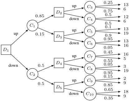
We consider a sequential decision problem under uncertainty represented by a decision tree T, i.e., an acyclic and connected graph including three types of nodes: a set DT of decision nodes (represented by squares), a set CT of chance nodes (represented by circles) and a set XT of outcome nodes (leaves). Each decision node represents a decision variable and the branches starting from that node correspond to the possible decisions (the domain of the variable). The branches starting from a chance node correspond to different possible events and are labelled by their probabilities. The leaves represent the possible outcomes (e.g., profits, time). An example of decision tree is given in Figure 1. The root of the tree is a decision node representing the initial decision to be made. The rank of the other decision nodes in the tree indicate the order in which decisions are made (from the left to the right). In the tree, the selection of an action at node Di is characterized by an edge (Di, A) where A is a child of Di. Note that this selection makes irrelevant all decision nodes outside from the tree rooted at A. For example, in the tree pictured in Figure 1, the decision up in D1 makes irrelevant nodes D4 and D5. In the tree, policies are characterized by the sequential selection of an action at every (relevant) decision node. Every policy can therefore be represented by a set of edges in the tree. For example, in Figure 1, policy π selecting up in nodes D1, D2 and D3 is represented by the following edges: {(D1,C1), (D2,C3), (D3,C5)}. Every policy induces a probability distribution on the leaves of the tree. This distribution can be represented by a lottery ℓ = (x1, p1; . . . ; xm, pm) yielding outcome xk with probability pk, where pk, k = 1, . . . ,m, are strictly positive and add up to one. For example, policy π corresponds to the lottery ℓ = (6, .6375; 13, .2275; 19, .135). In the tree depicted in Figure 1, there exist 8 policies leading to 8 distinct lotteries.
We adopt here the Bayesian theory of rational behavior under risk [Von Neumann and Morgenstern, 1947; Hammond, 1988]. The DM is assumed to be an expected utility maximizer and is consistent with the postulates of von Neuman and Morgenstern (vNM) theory. The DM's preferences over lotteries are therefore represented by the expected utility model defined by f(ℓ, u) = ∑mk=1 pku(xk) for any lottery ℓ = (x1, p1; . . . ; xm, pm), where u is the vNM utility function of the DM. A lottery ℓ is preferred to a lottery ℓ′ if and only if f(ℓ, u) ≥ f(ℓ′ , u). The set of policies inherits from the preferences defined over lotteries. Hence a policy is optimal in a tree T if the associated lottery maximizes function f over the set LT of all lotteries attached to the policies in T.
In this context, we want to elicit preferences in order to determine the preferred policy without resorting to explicit enumerations and comparisons. As a preliminary to elicitation, in the first part of the paper, we address the computation of possibly optimal lotteries under incomplete preference information (Section 2). This topic has been recently addressed in various contexts related to AI, including multi-agent decision making [Konczak and Lang, 2005; Xia and Conitzer, 2008; Roijers et al., 2014; Aziz et al., 2015], valued constraint satisfaction [Gelain et al., 2010; Marinescu et al., 2013] and multiobjective optimization [Benabbou and Perny, 2015b].
We address here a similar issue in the context of sequential decision making under risk. This work departs from previous studies in decision trees that consider partial preferences induced by imprecise probabilities, see e.g., [Kikuti et al., 2011]. Here probabilities are known and the incompleteness of preferences is only due to the imprecision of utilities. The second part of the paper is dedicated to preference elicitation (Section 3). We assume that the vNM utility u of the DM is initially unknown and we introduce a new approach interleaving the elicitation of u and the exploration of possibly optimal policies to determine an optimal policy in a decision tree. Finally, we introduce a representation of imprecise utilities using spline functions and we provide numerical tests showing the practical efficiency of the proposed approach (Section 4).
2 Computing Possibly Optimal Lotteries
We consider a situation where the DM's preferences are incomplete. The DM may have expressed some preference statements over various pairs of lotteries, but they are not sufficient to construct a precise vNM utility. These initial preference statements only induce some constraints on the space of utilities restricting the set U of admissible utility functions. Based on this partial information, we are interested in exploring the elements of POU(LT ), the set of possibly optimal lotteries in LT , i.e. lotteries that are f-optimal for at least one utility function in U. Formally, for any set L of lotteries:
This set can be constructed using the U-dominance relation ≻U defined as follows:
Definition 1. For any set L of lotteries and for any lottery ℓ0: L ≻U ℓ0 ⇔ ∀u ∈ U, ∃ℓ ∈ L, f(ℓ, u) > f(ℓ0, u).
For any set L of lotteries, we indeed have:
This result directly follows from Definition 1. It shows that POU(L) is exactly the set of non U-dominated lotteries in L. Note that, for any set L′ ⊆ L and for any lottery ℓ0 ∈ L, if L′ ≻U ℓ0 then L ≻U ℓ0; therefore, POU(L) = {ℓ ∈ L : not(L ≻U ℓ)}. As a consequnce, to conclude on whether a given lottery ℓ0 ∈ L is in POU(L) or not, it is sufficient to check if L ≻U ℓ0 holds (there is no need to enumerate and make the test for all subsets L′ ⊆ L). Moreover, we have:
This result which directly follows from Definition 1 allows one to check in polynomial time whether L ≻U ℓ0 is satisfied or not by solving a linear program, provided that U can be represented by a convex polyhedron (we will explain in Section 4 why this assumption is reasonable).
In order to compute POU(LT ), we now introduce a backward induction algorithm rolling back the tree from the leaves to the root. We assume that the root of the tree is a decision node and that the set DT of decision nodes in T is topologically sorted: if there exists a path fromnodeDi to nodeDj in the tree, then we necessarily have i < j. Starting from the last decision node in the topological order, one iteratively computes the set of non U-dominated lotteries attached to subpolicies rooted at decision nodes, until reaching the root. This idea is implemented in Algorithm 1. In this algorithm, each node Di keeps a set Li of lotteries attached to subpolicies rooted at that node (which is stored in the lotteries attribute). This set is computed by examining every child A of node Di. If A is a decision node, then all lotteries that are stored in A are inserted in Li. If A is a leaf of the tree, then the lottery (A, 1) yielding outcome A with probability 1 is inserted in Li. Otherwise, A is a chance node and all combinations of the lotteries stored in the descendants of A are inserted in Li. These combinations are computed by recursive calls to Combination from the initial call Combination(A), where p(A, Ak) denotes the probability on edge (A, Ak) (see Algorithm 2). Finally, only the non U-dominated elements of Li are stored in the lotteries attribute (see line 8). The following results will be used to prove the correctness of our algorithm:
Proposition 3 (Independence). For any lottery ℓ0 and any set L of lotteries, if L ≻U ℓ0 then, for any lottery ℓ′ and any λ ∈ (0, 1), we have: {λℓ+(1-λ)ℓ′ : ℓ ∈ L} ≻U λℓ0+(1-λ)ℓ′ .
This result directly derives from the fact that the DM is an EU-maximizer and that vNM independence holds in EU theory. Moreover, let Li be the set of lotteries attached to the policies rooted at node Di for i ∈ {1, . . . , |DT |}. We have:
Proposition 4. Let (Di,Dj) ∈ D2T be any pair of nodes such that Dj is a descendant of Di in T. Let ℓi be the lottery associated with a policy π rooted at Di and let ℓj be the lottery associated with the subpolicy of π rooted at Dj. If ℓj is Udominated in Lj then ℓi is U-dominated in Li.
Proof. Since ℓj is U-dominated in Lj, there exists a set L ⊆ Lj such that L ≻U ℓj. We want to prove that L′ ≻U ℓi holds for some set L′ ⊆ Li. Since Dj is a descendant of Di in the tree, there exists a unique path (A1, . . . ,An) from node Di to node Dj, with A1 = Di and An = Dj. If Ak ∈ DT for all k ∈ {1, . . . , n}, then we necessarily have ℓi = ℓj and L ⊆ Li. In that case, L ≻U ℓi follows from the hypothesis. Otherwise, ℓi is necessarily of the form ℓi = λℓj +(1-λ)ℓ′ , where λ = ∏k:Ak∈CT p(Ak,Ak+1) and p(Ak,Ak+1) is the probability labelling the edge (Ak,Ak+1). Since L ≻U ℓj by hypothesis, we obtain L′ ≻U ℓi by Proposition 3, where L′ = {λℓ + (1 -λ)ℓ′ : ℓ ∈ L} ⊆ Li.
Algorithm 1: Backward Induction.
Input: T: a decision tree; U: admissible utilities 1 for i = |DT |, . . . , 1 do 2 Li ← ∅; 3 for each edge (Di, A) in T do 4 if A ∈ DT then Li ← Li ∪ A.lotteries; 5 else if A ∈ CT then Li←Li ∪Combination(A); 6 else Li ← Li ∪ {(A, 1)}; 7 end 8 Di.lotteries ← {ℓ ∈ Li : not(Li ≻U ℓ)}; 9 end 10 return D1.lotteriesAlgorithm 2: Combination.
Input: A: a chance node 1 Let A1, . . . An denote the n children of node A; 2 for each edge (A,Ak) in T do 3 if Ak ∈ DT then L′k ←Ak.lotteries; 4 else if Ak ∈ CT then L′k ←Combination(Ak); 5 else L′k ← {(Ak, 1)}; 6 end 7 L← ∅; 8 for each (ℓ1, . . . , ℓn) ∈ L′1 × . . . ×L′n do 9 L←L∪ {∑nk=1 p(A,Ak)ℓk} 10 end 11 return LRelation ≻U also satisfies the following property:
Proposition 5 (Transitivity). For all lotteries ℓ0, ℓ1 and for all sets L,L′ of lotteries, if L ≻U ℓ1 and {ℓ1} ∪ L′ ≻U ℓ0 then L∪L′ ≻U ℓ0.
This follows directly from the transitivity of the preferences induced by the EU model. Moreover, we obviously have:
Proposition 6. For any set L of lotteries and any ℓ0 ∈ L, we have: ℓ0 ̸∈ POU(L) ⇒POU(L) ≻U ℓ0.
The last two results are now used to prove the following one:
Proposition 7. For any two sets L,L′ of lotteries, we have: POU(L) ⊆ L′ ⊆ L ⇒ POU(L′ ) ⊆ POU(L).
Proof. Let ℓ′ ∈ POU(L′ ). We want to prove that ℓ′ ∈ POU(L). Since ℓ′ ∈ POU(L′ ), we have not(L′′ ≻U ℓ′ ) for all L′′ ⊆ L′ (by (1)). Moreover, we have POU(L) ⊆ L′ by hypothesis; therefore, not(L′′ ≻U ℓ′ ) for all L′′ ⊆ POU(L). Now, we prove by contradiction that we have not(L′′ ≻U ℓ′ ) for all L′′ ⊆ L. Let us assume that there exists some L′′ 0 ⊆ L such that L′′ 0 ≻U ℓ′ . Since we proved that not(L′′ ≻U ℓ′ ) for all L′′ ⊆ POU(L), we have L′′ 0 ̸⊆ POU(L). Hence there exists some ℓ0 ∈ L′′ 0 such that ℓ0 ∈ L and ℓ0 ̸∈ POU(L). Then, using Proposition 6, we have POU(L) ≻U ℓ0. Moreover, since L′′ 0 ≻U ℓ′ , we derive POU(L) ∪ L′′ 0 \{ℓ0} ≻U ℓ′ by transitivity (see Proposition 5). Let L′′ 1 = POU(L) ∪ L′′ 0 \{ℓ0}. Note that we have POU(L) ⊆ L′′ 1 by definition. If there exists ℓ1 ∈ L′′ 1 such that ℓ1 ̸∈ POU(L), then we can iterate the reasoning to derive L′′ 2 ≻U ℓ′ where L′′ 2 = POU(L) ∪ L′′ 1 \{ℓ1}. Note that L′′ 2 = L′′ 1 \{ℓ1} since POU(L) ⊆ L′′ 1 and ℓ1 ̸∈ POU(L). Thus, we can further iterate to construct an embedded sequence L′′ 1 ⊃ . . . ⊃ L′′n = POU(L) such that L′′ k ≻U ℓ′ for all k ∈ {1, . . . , n}. Therefore, we have POU(L) ≻U ℓ′ . Moreover, POU(L) ⊆ L′ by hypothesis, which implies ℓ′ ̸∈ POU(L′ ) by Proposition 1. This yields a contradiction since ℓ′ ∈ POU (L′ ) by definition. Hence, there exists no L′′ 0 ⊆ L such that L′′ 0 ≻U ℓ′ . Moreover, ℓ′ ∈ L′ ⊆ L by hypothesis. Hence ℓ′ ∈ POU(L).
Proposition 8. Algorithm 1 returns the set POU(LT ).
Proof. Let LA denote the output of Algorithm 1. We have to prove that POU (LT ) ⊆ LA and LA ⊆ POU (LT ).
- POU(LT ) ⊆ LA: using Proposition 4, we know that only subpolicies leading to U-dominated policies are
deleted (in line 8). Since POU(LT ) is exactly the set of non U-dominated elements in LT (due to Proposition 1), POU (LT ) ⊆ LA holds.
- LA ⊆ POU(LT ): this inclusion is implied by Proposition 7 (with L = LT and L′ = LA). More precisely, we have POU(LT ) ⊆ LA ⊆ LT which implies POU(LA) ⊆ POU(LT ). Since POU(LA) = LA (due to line 8), we conclude that LA ⊆ POU (LT ).
Example 1. Coming back to Figure 1 and assuming that no preference information is available, relation ≻U eliminates up in D5 (edge (D5, C9)), down in D3 (edge (D3, C6)), down in D2 (edge (D2,C4)) and nothing in D4. This leads to three policies in D1: π1 = {(D1,C1), (D2,C3), (D3,C5)}, π2 = {(D1, C2), (D4, C7), (D5, C10)} and π3 = {(D1, C2), (D4,C8), (D5,C10)}. Relation ≻U eliminates no policy in D1. Hence POU(LT ) = {ℓ2, ℓ3, ℓ4}, where ℓi denotes the lottery associated to policy πi.
Algorithm 1 relies on the nice properties of ≻U that make possible to construct efficiently the optimal policies using dynamic programming. However, there exist instances of binary decision trees of depth d for which all policies are possibly optimal and correspond to disctinct lotteries. In such cases, the set of possibly optimal lotteries includes Θ(22d ) elements that obviously cannot be enumerated in polynomial time. This suggests inserting preference queries during the search so as to progressively reduce the number of possibly optimal lotteries until being able to determine a near-optimal lottery. The next section investigates this line.
3 Elicitation in Decision Trees
We propose to refine Algorithm 1 by interleaving preference elicitation and backward induction. The idea is to perform an implicit and progressive reduction of POU(LT ) by using new preferences statements to focus the search on the relevant lotteries. Collecting preference information during the search is made possible by the following straightforward result:
Proposition 9. For any U,U ′ such that U ′ ⊆ U, for any set L of lotteries and for any lottery ℓ0: L ≻U ℓ0 ⇒ L ≻U ′ ℓ0.
This proposition shows that new preference statements obtained during the search do not invalidate the pruning operations (based on relation ≻U) made so far while increasing pruning opportunities for the rest of the search.
In order to collect preference information, we use an adaptive elicitation approach based on regret minimization (as proposed in [Wang and Boutilier, 2003]) relying on the computations of pairwise max regrets (PMR), max regrets (MR) and minimax regrets (MMR) defined as follows:
- PMR(ℓ, ℓ′ , U ) = maxu∈U {f (ℓ′ , u) - f (ℓ, u)}
- MR(ℓ, LT , U) = maxℓ′∈LT PMR(ℓ, ℓ′ , U)
- MMR(LT , U) = minℓ∈LT MR(ℓ, LT , U)
The optimal lotteries for the minimax regret criterion are the elements of argminℓ∈LT MR(ℓ,LT ,U). By definition, the utility loss incurred by the choice of any of these lotteries is bounded above by the minimax regret value MMR(LT , U). This suggests progressively collecting preference statements from the DM until MMR(LT , U) drops below a given tolerance threshold δ ≥ 0. Ideally, we would like to ask preference queries until MMR(LT , U) = 0, which corresponds to the identification of an optimal lottery. However, to reduce the elicitation burden, it is more efficient to use a threshold δ > 0 representing the maximum admissible gap to optimality.
To determine a lottery ℓ ∈ LT with a MR below δ, we propose an interactive backward induction algorithm that generates preference queries to discriminate between the lotteries attached to the decision nodes (see Algorithm 3). We ask preference queries until MMR(Li,U) ≤ δ/η where η denotes the maximum number of decision nodes included in a path from the root to a leaf of the tree. This ensures that the MR value of the returned lottery is bounded above by δ (because any path from the root to a leaf includes at most η decision nodes). Contrary to Algorithm 1, only one lottery is stored in each decision node Di. This lottery is arbitrarily chosen among those minimizing MR(ℓ,Li,U) over the set Li of lotteries attached to node Di (see lines 15-16).
In order to reduce MMR(Li, U) at a given decision node Di, one may be tempted to ask the DM to compare two lotteries in Li and state which one she prefers (as in the Current Solution Strategy presented in [Boutilier et al., 2006]). However, lotteries associated with subpolicies in a decision tree are complex objects with multiple possible outcomes, which makes direct comparison cognitively difficult. We propose instead to ask the DM to compare lotteries of type ℓx = (x, 1) to lotteries of type ℓλ = (x⊤, λ; x⊥, 1 - λ), where x⊤ and x⊥ are respectively the best and worst possible outcomes. Note that we can impose u(x⊥) = 0 and u(x⊤) = 1 since vNM utilities are unique up to positive affine transformations. Hence f(ℓλ , u) = λu(x⊤) + (1 - λ)u(x⊥) = λ for all λ ∈ [0, 1]. Moreover, we have f(ℓx, u) = u(x) for all x ∈ XT . Therefore, if the DM prefers ℓx to ℓλ , then we derive the constraint u(x) ≥ λ; otherwise, we have u(x) ≤ λ. This shows that we must choose λ = (maxu∈U u(x) + minu∈U u(x))/2 to reduce the uncertainty attached to u(x) as much as possible in the worst-case scenario of answer. At each iteration step, we choose an outcome x ∈ ⋃ℓ∈Li S(ℓ) maximizing maxu∈U u(x) - minu∈U u(x), where S(ℓ) denotes the set of possible outcomes {x1, . . . , xm} of lottery ℓ = (x1, p1; . . . ; xm, pm). This choice enables to obtain interesting performance guarantees as shown below.
Proposition 10. For any set U of admissible utility functions and any set L of lotteries, if maxu∈U u(x) -minu∈U u(x)≤ δ/(2η) for all x∈ ⋃ℓ∈L S(ℓ), thenMMR(L,U)≤δ/η.
Proof. Let u∗ denote the actual vNM utility function of the DM. Let ℓ = (x1, p1; . . . ; xn; pn) be an element of arg maxℓ′∈L f (ℓ′ , u∗ ). We want to show that MR(ℓ, L, U)≤ δ/η. For all ℓ′ = (x′1 , p′1 ; . . . ; x′m; p′m) ∈ L, we have:
Thus, PMR(ℓ, ℓ′ , U) + f (ℓ, u∗ ) - f (ℓ′ , u∗ ) ≤ δ/η. Since f(ℓ, u∗ ) - f(ℓ′ , u∗ ) ≥ 0 by definition of ℓ, we obtain PMR(ℓ, ℓ′ , U)≤δ/η and so MR(ℓ, L, U)≤δ/η.
Input: T: a tree; U: admissible utilities: δ: a threshold 1 for i = |DT |, . . . , 1 do 2 Li ← ∅; 3 for each edge (Di, A) in T do 4 if A ∈ DT then Li ← Li ∪ A.lotteries; 5 else if A ∈ CT then Li←Li ∪Combination(A); 6 else Li ← Li ∪ {(A, 1)}; 7 end 8 Li ← {ℓ ∈ L : not(L ≻U ℓ)}; 9 while MMR(Li,U) > δ/η do 10 Select x ∈ argmax x′∈⋃ℓ∈Li S(ℓ){max u∈U u(x) - min u∈U u(x)}; 11 λ ← (maxu∈U u(x) + minu∈U u(x))/2; 12 Ask the DM to compare ℓx and ℓλ ; 13 Update U according to the answer; 14 end 15 Select one lottery ℓ in argminℓ′∈Li MR(ℓ′ ,Li,U); 16 Di.lotteries ← {ℓ}; 17 end 18 return D1.lotteriesProposition 11. Algorithm 3 has a time complexity of O(poly(nT , 1/δ)) and uses only O(poly(nT , 1/δ)) queries, where nT is the number of nodes in tree T.
Proof. On the number of queries: Initially, maxu∈U u(x) - minu∈U u(x) ≤ u(x⊤)-u(x⊥) = 1 for all outcomes x ∈ XT since u ∈ U is an increasing function. At each iteration step, the question asked in line 12 allows us to divide by two the range of possible values for u(x) for some x ∈ ⋃ℓ∈Li S(ℓ) such that maxu∈U u(x) -minu∈U u(x) > δ/(2η). Hence, for each outcome x in the tree, we need at most ⌈log2(2η/δ)⌉ queries to reduce the range from 1 to δ/(2η). We know that this is sufficient to obtain MMR(Li, U) ≤ δ/η at every decision node Di due to Proposition 10. Then, since we have |XT | ≤ nT outcomes and η ≤ nT , the overall number of queries is bounded above by nT ⌈log2(2nT /δ)⌉.
On the time complexity: we assume that U-dominance tests and PMR computations can be performed in polynomial time (w.r.t. nT ) using linear programming (this point will be justified in the next section). At each decision node Di, Algorithm 3 computes the set Li composed of all the lotteries attached to the mi children of Di (see lines 2-7); the U-dominated lotteries are then removed from Li (see line 8). Since only one lottery is stored in the lotteries attribute of each decision node, set Li necessarily includes at most mi elements. Hence, in the worst-case scenario, the computation of MMR(Li,U) requires to solve mi(mi - 1) PMR-optimization problems. Since mi ≤ nT and PMR-optimizations are performed in polynomial time (w.r.t. nT ), we know that all values MMR(Li,U) are computed in polynomial time (w.r.t. nT ). Moreover, at each decision node Di, the value MMR(Li, U) is computed exactly qi + 1 times, where qi is the number of queries generated at step i. Since we just proved that our algorithm uses only O(poly(nT , 1/δ)) queries in all, then it has a time complexity of O(poly(nT , 1/δ)).
Example 2. We illustrate Algorithm 3 on the tree of Figure 1 (with δ = 0.001). We assume that no preference information is initially available. In node D5, no preference query is needed since relation ≻U eliminates up. This is not the case in D4 where ≻U does not discriminate between up and down whose associated lotteries are ℓ = (5, 0.55; 16, 0.45) and ℓ′ = (3, 0.05; 19, 0.95). Since MMR({ℓ, ℓ′ },U) > δ/2, the DM is asked to compare lottery (5, 1) to lottery (x⊥, 0.5; x⊤, 0.5) where x⊥ = 0 and x⊤ = 20. If the DM prefers the latter, then U is updated by inserting the constraint u(5) ≤ 0.5. Now, MMR({ℓ, ℓ′ },U) ≤ δ/2 and up is eliminated. Nodes D3 and D2 are treated similarly as D5 but down is eliminated instead of up. As a result, in D1, we only obtain policies π1 and π3 (as defined in Example 1). Lottery ℓ1 is now U-dominated in D1 and therefore lottery ℓ3 is returned. The problem has been solved with a single query.
4 Implementation
To implement Algorithm 3 efficiently, we first discuss the representation of imprecise utility functions by convex polyhedra. Then, we will report some numerical results.
Representation of imprecise utilities. The first idea that probably comes to mind is to define a variable ux representing the value u(x) for every outcome x ∈ XT . With this representation, any preference statement comparing two lotteries translates into a linear inequality in variables ux, x ∈ XT . Hence the set U is a convex polyhedron. However, this representation has two drawbacks. First, beside the constraints imposed by the observed preferences, a number (still polynomial) of additional constraints is needed to enforce monotonicity of utilities (i.e. ux > uy whenever x > y). Moreover, the number of parameters to be learned grows with |XT |.
A more compact representation can be obtained if we define u as a spline function. Spline functions are piecewise polynomials whose elements connect with a high degree of smoothness. They are widely used in data interpolation due to their ability to approximate complex shapes [Ramsay, 1988]. Interestingly enough, spline functions can be generated by linear combinations of basis spline functions. This allows to reduce the elicitation of a spline function to the determination of its weights in the spline basis. In order to model utility functions which are non-decreasing functions of outcomes, one particularly appealing basis of spline functions is the basis of I-spline functions denoted Ii(x; k, t), i = 1, . . . ,m, where k is the order of the spline function (controlling the degree and the scope of polynomial pieces), t is a subdivision of their definition interval and m = |t|-k is the size of the spline basis. These functions are non-decreasing with respect to x. In this paper, we use I-spline functions of order 3 with a uniform subdivision of the unit interval (assuming that outcomes have been normalized to belong to the unit interval). This is a standard choice to keep a good controllability and flexibility because we keep low the degree of polynomials pieces while guaranteeing that adjacent pieces have matching first and second derivatives. Using the I-spline representation, the DM utility function writes: u(x) = ∑mj=1 bjIj(x; 3, t), bj ≥ 0, j = 1, . . . ,m. Assuming that outcomes are defined in the
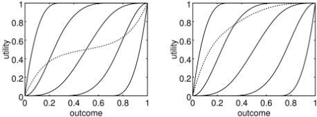
[0, 1] interval, individual utilities are normalized in order to have u(0) = 0 and u(1) = 1 by imposing that ∑mj=1 bj = 1.
In Figure 2, we give two examples of functions u (dashed lines) generated from a basis of functions Ij(x; 3, t), j = 1, . . . , 5 (solid lines), for a uniform subdivision of the interval. In the left part of the figure, the utility is defined from weights (0.3, 0.2, 0.0, 0.2, 0.3) whereas in the right part of the figure, the utility is defined from weights (0.5, 0.3, 0.2, 0.0, 0.0). Using only these five coordinates, we can generate an infinity of smooth functions covering or well approximating most functions. We might use a finer subdivision to cover even more complex functions including local irregularities.
The main advantage of this representation is to provide a compact definition of the parameter set. Indeed, only m variables are needed to characterize function u. This number is independent of the size of the tree. Moreover, although I-spline functions are not linear, it is worth noting that any preference statement of type "I prefer ℓ to ℓ′ " where ℓ = (x1, p1; . . . ; xq, pq) and ℓ′ = (x′1 , p′1 ; . . . ; x′r , p′r ) translates into a linear inequality in variables bj, j = 1, . . . ,m, which writes as follows:
Hence U is implicitly represented by a convex polyhedron defined as the set of all vectors (b1, . . . , bm) that are compatible with the available preference statements. Moreover, function u being defined as a convex combination of the Ispline basis functions, it is necessarily monotonic and we can get rid of any monotonicity constraint.
Numerical tests. Our elicitation strategy (see lines 9-14 in Algorithm 3) has been compared to the random strategy that consists in choosing outcome x and value λ at random at each iteration step. The MMR value reduces much more quickly with our strategy than with the random strategy. To give an example, for datasets with 100 (non stochastically dominated) lotteries, our strategy determines the best lottery after 15 queries on average while the MMR value with the random strategy is still above 30% of the initial regret at that moment.
Moreover, we report the results of numerical tests aiming to evaluate the performance of our interactive search procedure (Algorithm 3) on randomly generated instances of perfect binary trees (alternating decision nodes and chance nodes along each path). The depth d of the tree varies from 8 to
| δ = 0.1 | δ = 0.05 | |||||||
|---|---|---|---|---|---|---|---|---|
| Algorithm 3 | TS | Algorithm 3 | TS | |||||
| d | t | q | t | q | t | q | t | q |
| 8 | 0.15 | 12.1 | 0.90 | 7.2 | 0.22 | 17.0 | 1.69 | 8.9 |
| 10 | 0.39 | 16.4 | 11.94 | 8.6 | 0.42 | 21.0 | 14.46 | 10.9 |
| 12 | 1.21 | 19.7 | 725.51 | 9.4 | 1.20 | 22.3 | 2103.53 | 12.2 |
| 14 | 4.33 | 20.4 | - | - | 4.60 | 25.8 | - | - |
| 16 | 17.10 | 22.2 | - | - | 17.21 | 26.7 | - | - |
| 18 | 65.07 | 23.0 | - | - | 68.36 | 27.4 | - | - |
18 and the tolerance threshold from δ = 0.05 to 0.1. As a baseline for comparison, we consider the two stage procedure (named TS) that consists in computing L = POU(LT ) using Algorithm 1 and then asking preference queries until MMR(L,U) drops below δ (queries are generated as described in Section 3). Within both procedures, individual utilities are represented by spline functions. Starting from an empty set of preferences statements, simulated DMs answer to queries according to a randomly generated utility function. In Table 1, we report t (the computation times, in sec.) and q (the number of queries); the symbols "-" means that the procedure was still running after 5 hours 1 .
First, we see that Algorithm 3 is very efficient both in terms of number of queries and computation times. For example, for instances involving 229-1 policies (i.e. d = 18), it needs no more than 70 seconds and 23 queries to compute the result (for δ = 0.1). Moreover, Algorithm 3 is much faster than TS: when δ = 0.05 and d = 12, Algorithm 3 needs about 1 second to compute the result while TS takes more than 35 minutes. This shows that interleaving search and elicitation enables to drastically speed-up the determination of a nearoptimal solution in combinatorial domains.
5 Conclusion
We have proposed an adaptive utility elicitation procedure for the interactive selection of policies in sequential decision problems under risk. Our procedure interleaves preference queries with backward induction to progressively reduce the set of admissible utility functions and therefore the set of possibly optimal lotteries. The proposed procedure determines a near-optimal policy in polynomial time, using a polynomial number of preference queries. In addition to these theoretical guarantees, our numerical tests show the practical efficiency of this approach, especially when utility functions are represented by spline functions. This approach can easily be extended to the elicitation of additive utilities under risk, either in a multi-agent setting or in a multiattribute setting.
Acknowledgements
This work is supported by the ANR project 14-CE24-000701- Cocorico-CoDec.
1 The tests are performed on a Intel Core i7-4770 CPU with 15GB of RAM. LPs are optimized using the Gurobi solver.
@inproceedings{ijcai2017p637,
  title     = {Adaptive Elicitation of Preferences under Uncertainty in Sequential Decision Making Problems},
  author    = {Benabbou, Nawal and Perny, Patrice},
  booktitle = {Proceedings of the Twenty-Sixth International Joint Conference on
               Artificial Intelligence, {IJCAI-17}},
  publisher = {International Joint Conferences on Artificial Intelligence Organization},
  editor    = {Carles Sierra},
  pages     = {4566--4572},
  year      = {2017},
  month     = {8},
  note      = {Main track},
  doi       = {10.24963/ijcai.2017/637},
  url       = {https://doi.org/10.24963/ijcai.2017/637},
}
TY - CPAPER TI - Adaptive Elicitation of Preferences under Uncertainty in Sequential Decision Making Problems AU - Benabbou, Nawal AU - Perny, Patrice T2 - Proceedings of the Twenty-Sixth International Joint Conference on Artificial Intelligence, IJCAI-17 PB - International Joint Conferences on Artificial Intelligence Organization PY - 2017 SP - 4566 EP - 4572 DO - 10.24963/ijcai.2017/637 UR - https://doi.org/10.24963/ijcai.2017/637 ER -Copied
Machine-readable versions of this paper, for tools and AI agents:





