
Combining Models from Multiple Sources for RGB-D Scene Recognition
Proceedings of the Twenty-Sixth International Joint Conference on Artificial Intelligence. Main track. Pages 4523-4529.
https://doi.org/10.24963/ijcai.2017/631
Keywords
- Robotics and Vision: Robotics and Vision
- Robotics and Vision: Vision and Perception
Abstract
Depth can complement RGB with useful cues about object volumes and scene layout. However, RGB-D image datasets are still too small for directly training deep convolutional neural networks (CNNs), in contrast to the massive monomodal RGB datasets. Previous works in RGB-D recognition typically combine two separate networks for RGB and depth data, pretrained with a large RGB dataset and then fine tuned to the respective target RGB and depth datasets. These approaches have several limitations: 1) only use low-level filters learned from RGB data, thus not being able to exploit properly depth-specific patterns, and 2) RGB and depth features are only combined at high-levels but rarely at lower-levels. In this paper, we propose a framework that leverages both knowledge acquired from large RGB datasets together with depth-specific cues learned from the limited depth data, obtaining more effective multi-source and multi-modal representations. We propose a multi-modal combination method that selects discriminative combinations of layers from the different source models and target modalities, capturing both high-level properties of the task and intrinsic low-level properties of both modalities.
- [Banica and Sminchisescu, 2015] Dan Banica and Cristian Sminchisescu. Second-order constrained parametric pro- posals and sequential search-based structured prediction for semantic segmentation in rgb-d images. In The IEEE Conference on Computer Vision and Pattern Recognition (CVPR), June 2015.
- [Dash and Liu, 1997] Manoranjan Dash and Huan Liu. Fea- ture selection for classification. Intelligent Data Analysis, 1(1):131 -156, 1997.
- [Donahue et al., 2014] Jeff Donahue, Yangqing Jia, Oriol Vinyals, Judy Hoffman, Ning Zhang, Eric Tzeng, and Trevor Darrell. DeCAF: A deep convolutional activation feature for generic visual recognition. In International Conference on Machine Learning, (ICML), 2014.
- [Fan et al., 2008] Rong-En Fan, Kai-Wei Chang, Cho-Jui Hsieh, Xiang-Rui Wang, and Chih-Jen Lin. Liblinear: A library for large linear classification. Journal of Machine Learning Research (JMLR), 9:1871-1874, 2008.
- [Gupta et al., 2013] Saurabh Gupta, Pablo Arbeláez, and Ji- tendra Malik. Perceptual organization and recognition of indoor scenes from rgb-d images. In The IEEE Conference on Computer Vision and Pattern Recognition (CVPR), 2013.
- [Gupta et al., 2014a] Saurabh Gupta, Pablo Arbeláez, Ross Girshick, and Jitendra Malik. Indoor scene understanding with rgb-d images: Bottom-up segmentation, object detec- tion and semantic segmentation. International Journal of Computer Vision (IJCV), 112:133-149, 2014.
- [Gupta et al., 2014b] Saurabh Gupta, Ross Girshick, Ross Girshickand Pablo Arbeláez, and Jitendra Malik. Learn- ing rich features from rgb-d images for object detection and segmentation. In European Conference on Computer Vision (ECCV), 2014.
- [Gupta et al., 2016] Saurabh Gupta, Judy Hoffman, and Ji- tendra Malik. Cross modal distillation for supervision transfer. In The IEEE Conference on Computer Vision and Pattern Recognition (CVPR), June 2016.
- [Krizhevsky et al., 2012] Alex Krizhevsky, Ilya Sutskever, and Geoffrey E. Hinton. Imagenet classification with deep convolutional neural networks. In Neural Information Pro- cessing Systems (NIPS), pages 1106-1114, 2012.
- [Modrzejewski, 1993] Maciej Modrzejewski. Feature selec- tion using rough sets theory. In Proceedings of the Euro- pean Conference on Machine Learning, 1993.
- [Mucciardi and Gose, 1971] Anthony Mucciardi and Earl Gose. A comparison of seven techniques for choosing sub- sets of pattern recognition properties. IEEE Transactions on Computers, 20(9):1023-1031, September 1971.
- [Silberman and Fergus, 2011] Nathan Silberman and Rob Fergus. Indoor scene segmentation using a structured light sensor. In Computer Vision Workshops (ICCV Workshops), 2011 IEEE International Conference on, pages 601-608, November 2011.
- [Silberman et al., 2012] Nathan Silberman, Derek Hoiem, Pushmeet Kohli, and Rob Fergus. Indoor segmentation and support inference from rgbd images. In Proceedings of the 12th European Conference on Computer Vision - Volume Part V, ECCV'12, pages 746-760, Berlin, Heidel- berg, 2012. Springer-Verlag.
- [Song et al., 2015] Shuran Song, Samuel Lichtenberg, and Jianxiong Xiao. Sun rgb-d: A rgb-d scene understanding benchmark suite. In Computer Vision and Pattern Recog- nition (CVPR), 2015 IEEE Conference on, pages 567-576, June 2015.
- [Song et al., 2017] Xinhang Song, Luis Herranz, and Shuqiang Jiang. Depth cnns for RGB-D scene recog- nition: Learning from scratch better than transferring from rgb-cnns. In the Thirty-First AAAI Conference on Artificial Intelligence (AAAI), pages 4271-4277, 2017.
- [Wang et al., 2016] Anran Wang, Jianfei Cai, Jiwen Lu, and Tat-Jen Cham. Modality and component aware fea- ture fusion for rgb-d scene classification. In The IEEE Conference on Computer Vision and Pattern Recognition (CVPR), June 2016.
- [Xiao et al., 2013] Jianxiong Xiao, A. Owens, and A. Tor- ralba. Sun3d: A database of big spaces reconstructed using sfm and object labels. In Computer Vision (ICCV), 2013 IEEE International Conference on, pages 1625-1632, De- cember 2013.
- [Yang and Ramanan, 2015] Songfan Yang and Deva Ra- manan. Multi-scale recognition with dag-cnns. In The IEEE International Conference on Computer Vision (ICCV), December 2015.
- [Zhou et al., 2014] Bolei Zhou, Agata Lapedriza, Jianxiong Xiao, Antonio Torralba, and Aude Oliva. Learning deep features for scene recognition using places database. In Neural Information Processing Systems (NIPS), pages 487-495, 2014.
- [Zhu et al., 2016] Hongyuan Zhu, Jean-Baptiste Weibel, and Shijian Lu. Discriminative multi-modal feature fusion for rgbd indoor scene recognition. In The IEEE Conference on Computer Vision and Pattern Recognition (CVPR), June 2016.
References were extracted automatically from the PDF and may contain errors.
Full text extracted automatically from the PDF; figures, tables and equations may differ. The PDF is the version of record.
1 Introduction
RGB-D data has been widely used in computer vision tasks, using devices with both RGB and depth cameras, such as Microsoft Kinect. Depth data can help conventional RGB image recognition by providing additional information to better understand the spatial layout of the objects and regions in the scene. With the explosive growth of image datasets and the successful development of convolutional neural networks (CNNs) [Krizhevsky et al., 2012; Zhou et al., 2014; Donahue et al., 2014], the performance of RGB image recognition has been dramatically improved. However, training comparable RGB-D CNN models still remains challenging, due to the lack of suitable training data. Although transferring and fine tuning CNNs pretrained with large RGB datasets to the target depth data is helpful (in particular using the HHA
encoding[Gupta et al., 2013]), the intrinsic differences between RGB and depth modality limit RGB-D recognition.
Comparing to RGB image datasets, which can be collected by crawling data from the internet, collecting RGBD data is fairly complex, requiring a combination of RGBD sensors (e.g. Kinect) and a support device (e.g. laptop). Previous RGB-D datasets [Silberman and Fergus, 2011; Silberman et al., 2012; Xiao et al., 2013] contain much fewer categories and images than RGB counterparts. Recently, a larger RGB-D dataset SUN RGB-D [Song et al., 2015] was released providing more images to train more complex models, also showing that pretrained RGB CNNs can be used in this dataset with significantly less overfitting than with the previous reference dataset NYU2 [Silberman et al., 2012]. However, SUN RGB-D is still not large enough to train deep CNNs with size comparable to RGB ones (1K images compared to 2.5M in Places).
Thus, due to the lack of enough training data, recent approaches [Gupta et al., 2016; Wang et al., 2016; Zhu et al., 2016] have focused on transferring pretrained RGB CNN models and adapting them (typically fine tuning) with the target depth data. These approaches use the HHA encoding [Gupta et al., 2014b] for depth data. The HHA provides a color code which helps to intuitively visualize depth information, but more importantly, this encoding reveals some color patterns that somehow resembles RGB patterns. In [Wang et al., 2016] RGB and depth CNNs are obtained by fine tuning CNN models pretrained on large scale RGB datasets, then the resulting RGB and depth features are concatenated to train an SVM. RGB CNNs have also been used in other works to initialize depth CNNs which are further fine tuned using supervision transfer [Gupta et al., 2016] or distance loss between the outputs of RGB and depth CNNs [Zhu et al., 2016].
However, previous works suffer from some important limitations. First, fine tuning pre-trained RGB models with depth can adapt successfully the top layers of the CNN, but, due to the vanishing gradient problem, the bottom layers are barely modified, still remaining tuned to RGB modality. Reaching the bottom layers is key to learning depth modality-specific filters that capture low-level patterns. Without learning depthspecific filters for RGB-D combination, only similar patterns found in both RGB and depth modalities can be captured, while depth-specific, not found in the large RGB dataset are ignored. To illustrate this problem, Figure 1a and b show the activation maps of the first convolutional layer of PlacesCNN [Zhou et al., 2014] processing the same image but different modalities (i.e. cross-modal relations). As we can see, the captured patterns are often redundant to those already captured in the RGB modality (e.g. object edges) and often noisier, since the network is not trained for depth data. Second, these limited low-level depth representations are rarely considered, since the multi-modal combination is only performed at higher layers (e.g. fully connected layers) to exploit higherlevel correlations in previous works.
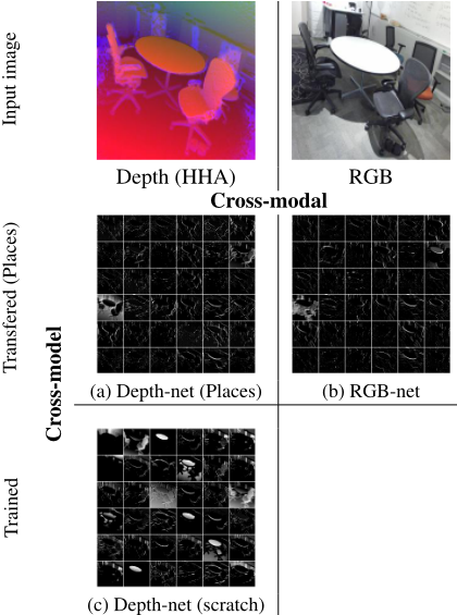
In contrast, activations in Figure 1c show depth-specific patterns which are very different from those in Figure 1a (i.e. cross-model relations). This model (see Section 2.1) has been trained only with depth data and thus can capture complementary information. In this way, it can provide truly depthspecific patterns which can complement RGB ones and help the overall model with this useful information.
Motivated by the need for better multi-modal features that capture modality-specific patterns, and also leveraging the vast knowledge already available in other source models such as Places-CNN, we propose a framework that combines models from multiple sources (i.e. Places for RGB and SUN RGB-D for depth) that are applied to be adapted and combined to the different modalities. In contrast to other works, this framework proposes a multi-source depth CNN
that effectively combines complementary models to capture modality-specific features. Moreover, by exploiting crossmodal and cross-model correlations, a layer selection algorithm is proposed to select discriminative combinations of layers from different models and modalities at different levels of abstraction.
2 Multi-source Multi-modal Framework
2.1 Base Models
Our framework processes RGB-D scene data, containing two modalities (RGB and depth encoded in HHA), and leverages three modality-specific models, one for RGB and two for depth. The three of them are based on the AlexNet architecture [Krizhevsky et al., 2012]. For convenience we introduce them at this point:
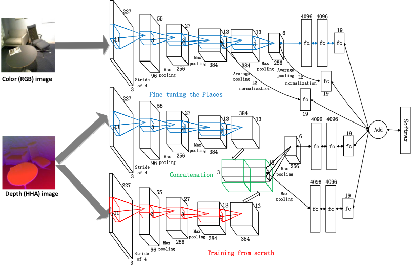
RGB-net: transferring from Places-CNN to RGB data. We fine tune Places-CNN model [Zhou et al., 2014] using the RGB images of the target RGB-D dataset. Since the original Places dataset contains large amount of scene data,which is in the same modality as the target RGB recognition task, the model will greatly benefit from transferring the parameters from Places-CNN.
Depth-net (Places): transferring from Places-CNN to depth data. Similar to RGB-net, we fine tune Places-CNN with the target depth images (in HHA format). In this case the adaptation is cross-modal, and with limited data, so the resulting model will basically adapt the top layers to the target data, while the low-level representations will remain unchanged and thus not tuned for depth data.
Depth-net (scratch): training directly from scratch with depth data. In order to learn a complementary depthspecific model, including low layers, we ignore Places and train AlexNet directly from scratch with the target depth data. To avoid overfitting we train first a truncated version (up to pool5) using patches (99×99 pixels sampled from the image 256×256 pixels), and then we fine tune the full network with full images.
2.2 Model Combination
We consider two types of CNN with different combinations of the three base CNN models, i.e., multi-source (MS) depth CNN that combines Depth-net (Places) and Depth-net (scratch) and multi-modal (MM) CNN that combines MSdepth-net and RGB-net.
Multi-source depth network (MS-depth-net). The most common method to represent depth is using a model similar to the one we refer to as Depth-net (Places). However, as we described earlier Depth-net (Places) and Depth-net (scratch) have different strengths and capture complementary patterns due to different modalities and different amounts in training data. For example, Depth-net (scratch) can capture better smooth gradients in HHA data due to horizontal and vertical surfaces, while Depth-net (Places) can still capture patterns present in both RGB and depth, such as borders, while also providing higher level compositional features for more abstract entities (e.g. objects, scenes) learned from the much larger dataset Places. Thus, the hypothesis is that by combining both models the result should be an improved depth representation that exploits the specific strengths of each model.
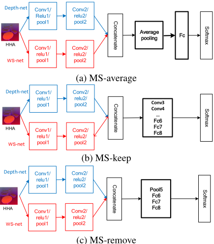
We regard each model as a different source model, and evaluate three different strategies to combine both models, illustrated in Fig. 2. The first one is simply concatenating the activations of a given layer in both models, followed by average pooling in a 1 × 1 × c tensor (i.e. a fixed c-dimensional vector). We refer this global representation as average (see Fig. 2a). For the classification task in the target dataset we further train a fully connected layer followed by softmax as classifier.
One drawback is that the spatial information is lost after average pooling, and the resulting network has fewer layers than the corresponding source models. We try another alternative in which after concatenating the activations, a single branch with the remaining layers (convolutional, pooling and fully connected) that are trained with the target depth data (see Fig. 2b). Since the number of parameters is higher and we only have limited data from the target dataset, we also evaluated another variation in which we remove the convolutional layers after concatenation (see Fig. 2c) to reduce the number of trainable parameters in the model. For simplicity, we refer to these two variants as keep and remove (convolutional layers), respectively.
Multi-modal network (MM-net). The full multi-modal network is shown in Fig. 3, where the (multi-source) depth network is further combined with the RGB branch, i.e. RGBnet. As shown in the figure, the different networks are combined by attaching fully connected layers as classifiers and their outputs are added before the softmax, similarly to DAGCNN [Yang and Ramanan, 2015]. A more discriminative combination method is introduced in the next section.
3 Layer Selection and Combination
3.1 Layer Selection
A common way to combine CNN models is directly concatenating the outputs of their respectively fully connected layers before the classifier (e.g. fc7 in AlexNet), then train a classifier and optionally fine tune the combined network. However, the activations from top layers may not be always the most suitable features for the particular task, especially for multi-modal representations, where the bottom layers are key to capture the modality-specific patterns. Moreover, it is often useful combining activations obtained at different layers of the same model [Yang and Ramanan, 2015].
In order to systematically explore combinations of features obtained from different layers of the same or different models, we introduce the problem of layer selection. We formulate the problem as selecting a set of layers L = {l1, l2, . . . lS}, where each candidate layer ls is selected by minimizing a weighted sum of the probability of error (POE) and the average correlation coefficient (ACC) [Mucciardi and Gose, 1971; Dash and Liu, 1997]. Particularly, POE is computed as the average class-error rate (i.e. top-1 average precision) on the validation set. Minimizing POE aims at selecting the most accurate layers. ACC is the average correlation coefficient (estimated on the validation data) between the confusion matrix of the model resulting from the selected layers at certain iteration and the confusion matrix of other model resulting after concatenating new candidate layers. Minimizing ACC aims at finding layers that increase the discriminative capability. We address the problem using an incremental formulation where the objective is to find the optimal set L as:
where P (l1, l2, . . . , lS) is the POE with the concatenation of the layers {l1, l2, . . . , lS}, C (lS | l1, l2, . . . , lS-1) is the ACC between the confusion matrices of the previous selected layers {l1, l2, . . . , lS-1} and after concatenating a new layer lS . Since this sum of POE and ACC does not have the Markov property, it cannot be optimized with a polynomial algorithm. Using brute-force search, in our typical setting with 3 CNN models with 7 layers each, there are 221 different combinations to be searched, which is too large to evaluate.
A greedy strategy to solve the problem is PRESET [Dash and Liu, 1997; Modrzejewski, 1993], which is based on the concept of "rough set". The algorithm first finds a reduct (i.e. a reduct R of LS that performs equally well as LS for the given task) and then removes all features/layers not selected in the reduct. It iteratively selects the features/layers for the reduct. In each iteration, all candidates are ranked using the weighed sum of POE and ACC, and the best candidate is selected.
However, this best first search algorithm is easily affected by the initial selection, and with a bad first choice the whole sequence of the selections may not find the best set of layers to combine. To trade off effectivity (brute force) and efficiency (best first search), we use the beam search (BS) algorithm. Rather than just selecting the first best layers in each iteration, a beam with a few candidate sets of layers is selected iteratively. At iteration t, the candidate sets U t are represented as:
where B is the beam number, and utb with b = 1, ..., B represents a possible set of selection until current iteration. At the next iteration t + 1, all candidates lv for v ∈ {candidates} are ranked using (1 - λ) P (utb , lv) + λC (lv | utb ) with current U t , and also the top B candidates are kept in the new set U t+1 . The search of one beam ends when no new candidate can be included.
3.2 Combination and Joint Training
Once the optimal set of layers L = {l1, l2, . . . lS} is obtained, we combine all of them in the joint CNN architecture, and fine tune it with pairs of RGB and depth images. A particular layer l indicates the combination point, i.e. the output of the corresponding layer of a particular model (e.g. conv4 of
| conv1 | conv2 | conv3 | conv4 | conv5 | fc6 fc7 | |
|---|---|---|---|---|---|---|
| RGB-net | 20.4 | 25.8 | 27.1 | 30.1 | 31.5 | 31.5 32.7 |
| Depth-net(PL) | 22.5 | 24.2 | 25.3 | 25.3 | 25.7 | 26.2 26.3 |
| Depth-net(SC) | 21.3 | 25.5 | 26.7 | 26.0 | 26.3 | 26.4 26.5 |
| MS-average | 25.0 | 27.7 | 27.1 | 27.0 | 27.1 | 28.0 27.9 |
| MS-keep | 21.0 | 24.8 | 27.4 | 28.0 | 29.5 | 29.8 29.4 |
| MS-remove | 22.2 | 27.7 | 28.5 | 29.4 | 29.5 | 29.8 29.4 |
PL: Places, SC: scratch
| Table 2: The best selections with different beam B | ||||
|---|---|---|---|---|
| B | Accuracy (%) | (1-λ)POE+λACC | ||
| Independent | MSMM | Independent | MSMM | |
| 1 | 35.6 | 36.1 | 0.661 | 0.657 |
| 2 | 36.0 | 36.4 | 0.657 | 0.654 |
| 3 | 36.3 | 36.8 | 0.654 | 0.650 |
| 4 | 36.3 | 36.8 | 0.654 | 0.650 |
Depth-net (Places)). The weights of that layer and the preceding ones are copied as initial weights to the corresponding layers of the joint model.
4 Experiments
4.1 Setup
We evaluate our approach in two datasets: NYU Depth Dataset version 2 (NYUD2) [Silberman et al., 2012] and
| Method | CNN model | Accuracy (%) | ||||
|---|---|---|---|---|---|---|
| RGB | Depth | RGB | Depth | RGB-D | ||
| Baseline (concatenate fc7) | Places-CNN RGB-net | Places-CNN Depth-net (PL) | - - | 35.4 41.5 | 30.9 37.5 | 39.1 45.4 |
| Two CNNs (concat fc7+FT) | RGB-net RGB-net | Depth-net (PL) - | - Depth-net (SC) | 41.5 41.5 | 37.5 37.2 | 48.5 48.3 |
| Multi-source depth Three CNNs (concat. fc7+FT) Layer selection (independent) Layer selection (MSMM) Layer selection (MSMM+wSVM) | - RGB-net RGB-net RGB-net | Depth-net (PL) Depth-net (PL) Depth-net (PL) | Depth-net (SC) Depth-net (SC) Depth-net (SC) | - - - - | 40.1 - - - - | - 49.8 50.6 |
| Depth-net (PL) + (SC) | 51.2 | |||||
| et | - 37.0 | 52.3 | ||||
| RGB-net Zhu | Depth-net (PL) + (SC) al.[Zhu et al., 2016] | - | - | 41.5 | ||
| State-of-the-art | Wang | et al.[Wang et al., 2016] Song et al.[Song et al., 2017] | 40.4 | 36.3 - | 48.1 52.4 | |
PL: Places, SC: scratch. FT: fine tuning. Proposed models are in bold.
SUN RGB-D [Song et al., 2015]. The former is relatively small, consisting of 27 indoor categories. Following the original training/test split (795/654 images) [Silberman et al., 2012], all 27 categories are reorganized into 10 categories, where some of categories with few images are combined into a joint category "other". The latter contains 40 categories with 10335 RGB-D images. Following the publicly available split in [Song et al., 2015; Wang et al., 2016], the 19 most common categories are selected, consisting of 4845/4659 images for training/test, where the training set consists of a split of 2393/2452 images for training/validation. The split is provided in the toolbox of SUN RGB-D dataset [Song et al., 2015]. All depth images are encoded to HHA images using the code in [Gupta et al., 2014b].
We train SVM [Fan et al., 2008] classifiers using the output of the last fully connected layer as input, as done in most state-of-the-art approaches. We include a variant (wSVM) in which we use class-specific weights to compensate class imbalance. Following [Song et al., 2015], we report the average class accuracy in both datasets.
4.2 Analysis
In this subsection, all the evaluations are conducted on the training and validation set of SUN RGB-D dataset, consisting of 2393 and 2452 images, respectively.
Ablation study of the base models. We evaluate how discriminative are the different layers of the different base models on their respective modalities by training SVMs and measuring the average class accuracy (see Table 2). The best individual performance is achieved with fc7, fc7 and conv3 for RGB-net, Depth-net (Places) and Depth-net (scratch), with a more significant increase of accuracy with deeper features in models transferred from Places, while Depth-net (scratch) suffers from overfitting in higher layers. Table 2 also shows different behaviours for different modalities and models. In the case of RGB-net, evaluated with RGB images, bottom layers perform poorly while higher layers gradually increase the performance. This shows the power of transferring a model pretrained with large data (Places) when applied on RGB data, and also that RGB modality requires deeper models. Applied on the depth modality (Depth-net (Places)), the behaviour is similar but with much more limited gains in deeper layers, showing that cross-modal transfer is of limited help. Similar performance can be obtained without resorting to Places, using directly depth data (i.e. Depth-net (scratch)). This also suggests that the depth modality is less complex than the RGB modality (e.g. no textures in depth data) and thus deeper models may not increase the performance significantly.
Multi-source depth models. We also evaluated the three strategies described in Fig. 2, with the results shown in Table 1. Combining Depth-net (Places) and Depth-net (scratch) performs consistently better than either of the source models independently. This happens consistently for all the layers and using either of the three combination strategies, suggesting that both source models capture complementary properties of the depth data, and showing the effectivity of the proposed approach. In general, MS-keep and MS-remove perform better than MS-average, except for conv1 (very shallow model). This suggests that keeping some rough spatial information when combining modalities is helpful for scene recognition. Particularly, MS-remove outperforms the other two strategies for most layers, benefiting from a better tradeoff between the amount of parameters and amount of training data than MS-keep.
Finally, it is worth noticing that multi-source (MS) models outperformRGB-net for lower layers (conv1 to conv3), while RGB-net outperforms them at higher layers, suggesting that for the final multi-modal model we should combine features selected from different layers of different models.
Layer selection and multi-modal combination. We empirically set λ = 0.1 and consider two settings. In a first experiment : independent (in Table 2), where layers are selected only from the three base models. We obtained the best results for beam sizes of B = 3 and 4. The best selection paths are reported in Table 2 (there are several possible paths for B > 1). Fig. 4a shows the layer selected and added at each
| Method | CNN model | Accuracy (%) | ||
|---|---|---|---|---|
| RGB | Depth | |||
| Baseline (concatenate fc7) | RGB-net | Depth-net (PL) | - | 45.4 |
| Three CNNs (concat. fc7+FT) Layer selection (independent) Layer selection (MSMM) Layer selection (MSMM+wSVM) | RGB-net RGB-net RGB-net RGB-net | Depth-net (PL) Depth-net (PL) Depth-net Depth-net | Depth-net (SC) Depth-net (SC) (PL) + (SC) (PL) + (SC) | 63.9 64.3 65.1 66.7 |
| State-of-the-art | Gupta et al.[Gupta et al., 2014a] Wang et al.[Wang et al., 2016] Song et al.[Song et al., 2017] | 45.4 63.9 65.8 | ||
PL: Places, SC: scratch. Proposed models in bold.
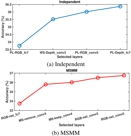
iteration, and how the performance progressively increases. A second experiment (multi-source multi-modal -MSMM-) shows similar trends and slightly better results (see Table 2 and Fig. 4b) when allowing layers from RGB-net, and the multi-source models MS-keep and MS-remove. Observe that in both experiments the algorithm always selects first features from a top layer from RGB and a lower layer from depth.
4.3 Overall Performance
We compare our method to the state-of-the-art approaches [Zhu et al., 2016; Wang et al., 2016; Song et al., 2017] on SUN RGB-D and NYUD2. For SUN RGB-D, we follow the public split, consisting of 4845/4659 images for training/test. In the case of NYUD2 we fine tune this pretrained model.
The comparisons are reported in Table 3, where the proposed multi-source model for depth modality combines two models, improving the performance up to 40.1%. The proposed layer selection algorithm also improves over simple concatenation of the three networks, with the multi-source variant (MSMM) achieving the best performance (with an additional gain if we address the imbalanced in the dataset with wSVM). Our method outperforms other approaches [Zhu et al., 2016; Wang et al., 2016], benefiting from capturing the depth specific patterns and a better feautre combination method. Song et al. [Song et al., 2017] propose to train CNN models with simple but effective architecture for depth data and concatenate RGB and depth models with fc7 output, obtaining similar results as our MSMM model. Compared to the proposed MS-net model, that depth model lacks of the considering general patterns shared RGB and depth data.
Table 4 shows the results on NYUD2. Our results also outperform the baseline and the related works. Note that, [Banica and Sminchisescu, 2015] reports a very high accuracy for NYUD2, however, the authors in [Wang et al., 2016] re-implement that method, but obtain much lower accuracy.
5 Conclusion
Different modalities provide complementary information to improve RGB-D recognition. Similarly, different models can capture complementary aspects within the same modality. For instance, we showed how Depth-net (scratch), a network trained from scratch can capture valuable low-level depthspecific patterns that cannot be captured by just fine tuning RGB-specific models (e.g., Depth-net (Places)). Moreover, it can complement other higher-level RGB-specific and depthspecific features. In this paper we propose a framework to combine features from multiple modality-specific models, including layer selection and joint fine tuning, which outperforms significantly current state-of-the-art.
Acknowledgments
This work was supported in part by the National Natural Science Foundation of China under Grant 61532018 and 61322212, in part by the Beijing Municipal Commission of Science and Technology under Grant D161100001816001, in part by the Lenovo Outstanding Young Scientists Program, in part by National Program for Special Support of Eminent Professionals and National Program for Support of Topnotch Young Professionals. This work was supported by the National Postdoctoral Program for Innovative Talents under Grant BX201700255. This work was partly supported by the EU under the Marie Sklodowska-Curie grant 665919.
@inproceedings{ijcai2017p631,
  title     = {Combining Models from Multiple Sources for RGB-D Scene Recognition},
  author    = {Song, Xinhang and Jiang, Shuqiang and Herranz, Luis},
  booktitle = {Proceedings of the Twenty-Sixth International Joint Conference on
               Artificial Intelligence, {IJCAI-17}},
  publisher = {International Joint Conferences on Artificial Intelligence Organization},
  editor    = {Carles Sierra},
  pages     = {4523--4529},
  year      = {2017},
  month     = {8},
  note      = {Main track},
  doi       = {10.24963/ijcai.2017/631},
  url       = {https://doi.org/10.24963/ijcai.2017/631},
}
TY - CPAPER TI - Combining Models from Multiple Sources for RGB-D Scene Recognition AU - Song, Xinhang AU - Jiang, Shuqiang AU - Herranz, Luis T2 - Proceedings of the Twenty-Sixth International Joint Conference on Artificial Intelligence, IJCAI-17 PB - International Joint Conferences on Artificial Intelligence Organization PY - 2017 SP - 4523 EP - 4529 DO - 10.24963/ijcai.2017/631 UR - https://doi.org/10.24963/ijcai.2017/631 ER -Copied
Machine-readable versions of this paper, for tools and AI agents:





