
Reduction Techniques for Model Checking and Learning in MDPs
Proceedings of the Twenty-Sixth International Joint Conference on Artificial Intelligence. Main track. Pages 4273-4279.
https://doi.org/10.24963/ijcai.2017/597
Keywords
- Multidisciplinary Topics and Applications: Validation and Verification
- Uncertainty in AI: Sequential Decision Making
- Planning and Scheduling: Markov Decisions Processes
- Uncertainty in AI: Uncertainty in AI
Abstract
Omega-regular objectives in Markov decision processes (MDPs) reduce to reachability: find a policy which maximizes the probability of reaching a target set of states. Given an MDP, an initial distribution, and a target set of states, such a policy can be computed by most probabilistic model checking tools. If the MDP is only partially specified, i.e., some prob- abilities are unknown, then model-learning techniques can be used to statistically approximate the probabilities and enable the computation of the de- sired policy. For fully specified MDPs, reducing the size of the MDP translates into faster model checking; for partially specified MDPs, into faster learning. We provide reduction techniques that al- low us to remove irrelevant transition probabilities: transition probabilities (known, or to be learned) that do not influence the maximal reachability probability. Among other applications, these reductions can be seen as a pre-processing of MDPs before model checking or as a way to reduce the number of experiments required to obtain a good approximation of an unknown MDP.
- [Aspnes and Herlihy, 1990] James Aspnes and Maurice Herlihy. Fast randomized consensus using shared memory. J. of Algo- rithms, 11(3):441-461, September 1990.
- [Baier and Katoen, 2008] Christel Baier and Joost-Pieter Katoen. Principles of model checking. MIT Press, 2008.
- [Bernstein et al., 2002] Daniel S. Bernstein, Robert Givan, Neil Im- merman, and Shlomo Zilberstein. The complexity of decentral- ized control of Markov decision processes. Math. Oper. Res., 27(4):819-840, November 2002.
- [Brafman and Tennenholtz, 2003] Ronen I. Brafman and Moshe Tennenholtz. R-max -a general polynomial time algorithm for near-optimal reinforcement learning. J. Mach. Learn. Res., 3:213- 231, March 2003.
- [Brázdil et al., 2014] Tomás Brázdil, Krishnendu Chatterjee, Martin Chmelik, Vojtech Forejt, Jan Kretínský, Marta Z. Kwiatkowska, David Parker, and Mateusz Ujma. Verification of Markov decision processes using learning algorithms. In ATVA, volume 8837 of LNCS, pages 98-114, 2014.
- [Ciesinski et al., 2008] Frank Ciesinski, Christel Baier, Marcus Größer, and Joachim Klein. Reduction techniques for model checking Markov decision processes. In QEST, pages 45-54, 2008.
- [Condon, 1992] Anne Condon. The complexity of stochastic games. Inf. Comput., 96(2):203-224, 1992.
- [Courcoubetis and Yannakakis, 1995] Costas Courcoubetis and Mi- halis Yannakakis. The complexity of probabilistic verification. J. ACM, 42(4):857-907, 1995.
- [De Alfaro, 1997] Luca De Alfaro. Formal verification of proba- bilistic systems. PhD thesis, Stanford University, 1997.
- [Dehnert et al., 2017] Christian Dehnert, Sebastian Junges, Joost- Pieter Katoen, and Matthias Volk. A storm is coming: A modern probabilistic model checker. In CAV, 2017.
- [Ding et al., 2014] X. Ding, S. L. Smith, C. Belta, and D. Rus. Op- timal control of Markov decision processes with linear temporal logic constraints. IEEE Trans. on Automatic Control, 59(5):1244- 1257, May 2014.
- [Fu and Topcu, 2014] Jie Fu and Ufuk Topcu. Probably approxi- mately correct MDP learning and control with temporal logic constraints. In RSS, 2014.
- [Haddad and Monmege, 2014] Serge Haddad and Benjamin Mon- mege. Reachability in mdps: Refining convergence of value itera- tion. In Joël Ouaknine, Igor Potapov, and James Worrell, editors, RP, volume 8762 of LNCS, pages 125-137. Springer, 2014.
- [Kaelbling et al., 1996] Leslie Pack Kaelbling, Michael L. Littman, and Andrew W. Moore. Reinforcement learning: A survey. JAIR, 4:237-285, 1996.
- [Kawaguchi, 2016] Kenji Kawaguchi. Bounded optimal exploration in MDP. In AAAI, pages 1758-1764, 2016.
- [Kearns and Singh, 2002] Michael Kearns and Satinder Singh. Near- optimal reinforcement learning in polynomial time. Machine Learning, 49(2):209-232, 2002.
- [Kolobov et al., 2011] Andrey Kolobov, Mausam, Daniel S. Weld, and Hector Geffner. Heuristic search for generalized stochastic shortest path mdps. In Fahiem Bacchus, Carmel Domshlak, Stefan Edelkamp, and Malte Helmert, editors, ICAPS. AAAI, 2011.
- [Kolter and Ng, 2009] J. Z. Kolter and Andrew Y. Ng. Near- bayesian exploration in polynomial time. In Andrea P. Danyluk, Lon Bottou, and Michael L. Littman, editors, ICML, page 65, 2009.
- [Kwiatkowska et al., 2001] Marta Z. Kwiatkowska, Gethin Norman, and Roberto Segala. Automated verification of a randomized distributed consensus protocol using Cadence SMV and PRISM. In CAV, pages 194-206, 2001.
- [Kwiatkowska et al., 2004] Marta Z. Kwiatkowska, Gethin Norman, David Parker, and Jeremy Sproston. Performance analysis of probabilistic timed automata using digital clocks. In FORMATS, pages 105-120, 2004.
- [Kwiatkowska et al., 2011] Marta Z. Kwiatkowska, Gethin Norman, and David Parker. PRISM 4.0: Verification of probabilistic real- time systems. In Ganesh Gopalakrishnan and Shaz Qadeer, editors, CAV, volume 6806 of LNCS, pages 585-591. Springer, 2011.
- [Lacerda et al., 2015] Bruno Lacerda, David Parker, and Nick Hawes. Optimal policy generation for partially satisfiable co- safe LTL specifications. In IJCAI, pages 1587-1593, 2015.
- [Lahijanian et al., 2010] M. Lahijanian, J. Wasniewski, S. B. Ander- sson, and C. Belta. Motion planning and control from temporal logic specifications with probabilistic satisfaction guarantees. In ICRA, pages 3227-3232, 2010.
- [Littman, 1996] Michael L. Littman. Algorithms for Sequential De- cision Making. PhD thesis, Brown University, 1996.
- [Papadimitriou and Tsitsiklis, 1987] Christos H. Papadimitriou and John N. Tsitsiklis. The complexity of Markov Decision Processes. Math. Oper. Res., 12:441-450, 1987.
- [Puterman, 2005] Martin L. Puterman. Markov Decision Processes. Wiley-Interscience, 2005.
- [Russell and Norvig, 2010] Stuart J. Russell and Peter Norvig. Arti- ficial Intelligence -A Modern Approach (3. internat. ed.). Pearson Education, 2010.
- [Russell et al., 2015] Stuart J. Russell, Daniel Dewey, and Max Tegmark. Research priorities for robust and beneficial artificial intelligence. AI Magazine, 36(4), 2015.
- [Steinmetz et al., 2016] Marcel Steinmetz, Jörg Hoffmann, and Olivier Buffet. Goal probability analysis in probabilistic planning: Exploring and enhancing the state of the art. JAIR, 57:229-271, 2016.
- [Strehl et al., 2009] Alexander L. Strehl, Lihong Li, and Michael L. Littman. Reinforcement learning in finite MDPs: PAC analysis. J. Mach. Learn. Res., 10:2413-2444, 2009.
- [Svorenová et al., 2013] María Svorenová, Ivana Cerna, and Calin Belta. Optimal control of MDPs with temporal logic constraints. In CDC, pages 3938-3943, 2013.
- [Valiant, 2013] Leslie Valiant. Probably Approximately Correct: Nature's Algorithms for Learning and Prospering in a Complex World. Basic Books, 2013.
- [Wen and Topcu, 2016] Min Wen and Ufuk Topcu. Probably ap- proximately correct learning in stochastic games with temporal logic specifications. In Subbarao Kambhampati, editor, IJCAI, pages 3630-3636, 2016. IJCAI
References were extracted automatically from the PDF and may contain errors.
Full text extracted automatically from the PDF; figures, tables and equations may differ. The PDF is the version of record.
1 Introduction
Markov decision processes (MDPs) are one of the most widely used tools for modelling decision-making under uncertainty [Littman, 1996; Papadimitriou and Tsitsiklis, 1987]. They are widely used in areas of planning [Russell and Norvig, 2010; Ding et al., 2014], model-based reinforcement learning [Strehl et al., 2009], formal verification [Baier and Katoen, 2008], robotics [Lahijanian et al., 2010], and control [Bernstein et al., 2002]. Arguably the most fundamental question one can ask in an MDP is to maximize the probability of reaching some target set of states from a set of initial states. That is, to compute the maximal reachability probability and a policy which - when implemented on the MDP - achieves that probability. In the artificial intelligence planning community, this problem is also known as MAXPROB (see, e.g., [Kolobov et al., 2011; Steinmetz et al., 2016]). A sample instance of the associated decision problem is as follows: "is there a policy to ensure the probability of reaching state t from state s is at least 10%?" More elaborate objectives defined with respect to reward or cost functions have also been considered in the literature [Puterman, 2005]. It can, however, be cumbersome to map complex goals to an appropriate reward structure in an MDP and thus find a control policy. To this end, linear temporal logic (LTL) has been commonly used as a way to formally specify high-level goals (see, e.g., [Svorenov´a et al., 2013; Lacerda et al., 2015]). It is known that maximizing the probability of satisfying several objectives, notably LTL objectives, reduces to a reachability objective [Baier and Katoen, 2008].
In this paper we develop MDP reduction techniques that preserve the maximal reachability probability. We first discuss why such reductions are needed.
Need for reductions in model checking. Model checking is a technique to formally verify properties of a model of a system against a formal specification, given, for instance, as an LTL formula [Courcoubetis and Yannakakis, 1995]. The advantage of model checking is that it provides an automated way for the user to verify if their specification holds in a model. Given an MDP, initial states, and a target set of states, model checking tools are able to compute the maximal reachability probability in time polynomial in the size of the MDP [Kwiatkowska et al., 2011; Dehnert et al., 2017].
Unfortunately, model checking is a model-based technique: it assumes the MDP will be given in a completely specified manner, i.e. all transition probabilities are assumed to be known in advance. In practice, these values often come from simulations or they are estimated by hand. If the accuracy of these values is unknown, then the result of model checking carries no relevant insight. Even if the transition probabilities have some guaranteed probability of being accurate, the guarantees provided by model checking will depend on both the precision and confidence parameters: the output will be only probably approximately correct (PAC) [Valiant, 2013].
One way to mitigate these weaknesses is to determine which transition probabilities affect the maximal reachability probability. It is known that not all transition probabilities impact the maximal reachability probability [Ciesinski et al., 2008; Br´azdil et al., 2014]. If some transition probabilities are irrelevant, then the guarantees on the outcome of the model checking process do not depend on the precision or confidence related to those values.
Need for reductions in learning. Another way to deal with partially specified MDPs is to use learning techniques [Kaelbling et al., 1996]. In this approach, and in order to obtain a PAC output, the model (i.e., its transition probabilities) are learned up to some precision with some desired confidence and then the MDP is processed [Wen and Topcu, 2016; Fu and Topcu, 2014]. A drawback of learning is that it requires a large number of samples - and, in turn, a large amount a time - to learn the transition probabilities with desirable precision and confidence parameters [Kawaguchi, 2016; Kolter and Ng, 2009; Russell et al., 2015]. This is especially the case for PAC learning algorithms like R-max [Brafman and Tennenholtz, 2003] and E3 [Kearns and Singh, 2002]. While these techniques provide attractive theoretical guarantees on optimality, they require practically excessive amounts of sampling and exploration [Kawaguchi, 2016; Kolter and Ng, 2009; Russell et al., 2015].
Here, it is natural to ask which transition probabilities one really has to learn and which ones can be left unexplored. If some transition probabilities are known to have no effect on the maximal reachability probability, then they can be omitted from the learning phase without affecting the guarantees on the output. We show that if the objective can be reduced to reachability, then the entire MDP need not be sampled and the MDP can be reduced to shorten necessary learning time and still provide the same guarantees.
Our contribution. We provide reduction techniques for MDPs to allow for more efficient reachability analysis and learning without sacrificing any correctness. In other words, given an MDP, initial states, and target states, we compute - in polynomial time - a smaller MDP with equivalent maximal reachability probability. We do this by removing distributions - state-action pairs and the resulting transitions enabled with non-zero probability - in the MDP that do not affect the maximal probability of reaching a target set of states from some initial states. More precisely, our algorithm uses the graph structure of the MDP (and can thus be used even if all the probabilities are unknown) to determine if some distributions are 'better' than others. We then use this information to remove sub-optimal actions (and, hence, distributions) from the MDP. We illustrate the reductions using small examples and show that we achieve reductions on MDPs with no end components and unique extremal probability states (these notions will be made precise in the sequel).
In two case studies from the well-known probabilistic model checking tool PRISM, the reduction in the size of the MDPs obtained by applying our techniques far outperforms current reduction techniques. We also test the proposed techniques on a model-based learning application with a classical gridworld test setup and observe a large reduction in learning time.
Related work. Reductions in MDPs have been investigated in formal verification. In [Ciesinski et al., 2008], the authors collapse end components and states from which the probability of satisfying the specification is 0 or 1. These will be presented in Sec. 3. The same techniques were also mentioned in [Br´azdil et al., 2014], where learning techniques are introduced to aid model checking MDPs. The authors also provide an algorithm to compute end components on the fly in the case where they are not known beforehand. We assume, however, that the graph structure of the MDP is known beforehand and hence all end components can be computed.
Structure. In Sec. 2, we provide the definitions and notation that will be followed in the paper. We present the known reduction techniques from related works in Sec. 3, followed by our novel techniques in Sec. 4. In Sec. 5, we present experiments where the reductions were applied on established model checking case studies from the PRISM tool as well as learning in a gridworld. We conclude and provide future directions in Sec. 6.
2 Preliminaries
We follow notation from [Littman, 1996; Puterman, 2005].
2.1 Markov Decision Processes
We denote by D(X) the set of all probability distributions on a finite set X, i.e. all functions f : X → [0, 1] such that ∑x∈X f(x) = 1. For f ∈ D(X) we denote by supp(f) the support of f. That is, the set {x ∈ X | f(x) > 0}.
Definition 1. An MDP is a tuple M = (S,A, δ) where S is a finite set of states, A is a finite alphabet of actions, δ : S × A → D(S) is a (partial) probabilistic transition function that assigns to a state s and an action a ∈ A a probability distribution over the successor states. We abbreviate δ(s, a)(s′ ) by δ(s′ |s, a).
Pictorially, the states of an MDP will be represented by circles; a distribution δ(s, a), by an arrow leaving state s with multiple heads - one per state s′ ∈ supp(δ(s, a)) - having its tail labelled with a and every head pointing to s′ with the value δ(s′ |s, a).
Same-support functions. Two probabilistic transition functions δ, δ′ are said to have the same support if supp(δ(s, a)) = supp(δ′ (s, a)) holds for all pairs (s, a) ∈ S × A. We write supp(δ) = supp(δ′ ) to denote this.
Runs and policies. A run from state s0 is a (possibly infinite) sequence ϱ = s0a0s1a1s2a2 . . . of states and actions such that for all i ≥ 0 we have δ(si+1|si, ai) > 0. A policy corresponds to a way of selecting actions based on the history of states and actions. We focus on deterministic stationary policies, since these are known to be sufficient for reachability probability optimization [Condon, 1992; Puterman, 2005]. Formally, a (deterministic stationary) policy is a function π : S → A which assigns to every state an action.
A run ϱ is consistent with a policy π if it can be obtained by extending its finite prefixes using π. Formally, ϱ = s0a0s1a1 . . . is consistent with π if for all i ≥ 0 we have that ai = π(si) and δ(si+1|si, ai) > 0.
Reachability probability. Given an initial distribution ι ∈ D(S), a policy π, and a target set of states T ⊆ S, the reachability probability P δ,π ι [Reach(T)] of π is the probability that a run starting from a state s, sampled from ι, and consistent with π will reach a state from T. This definition can be formalized by a standard construction of a probability measure induced by π over the set of all runs (see, e.g., [Puterman, 2005]). The maximal reachability probability is Valδι (T ) := maxπ P δ,π ι [Reach(T)].
Irrelevant distributions. For every initial distribution ι and target set T , we are interested in the set of state-action pairs
(s, a) ∈ S × A for which changing the distribution δ(s, a) -without changing its support -will not change the value Valδι (T). Formally, we consider an arbitrary probabilistic transition function δ′ such that: (i) δ(t, b) = δ′ (t, b) for all (t, b) ̸= (s, a) and (ii) supp(δ(s, a)) = supp(δ′ (s, a)). We say δ(s, a) is irrelevant if, for all such δ′ , it holds that Valδ′ ι (T) = Valδι (T) -where Valδ′ ι (T) refers to the maximal reachability probability in the MDP (S, A, δ′ ).
3 Well-Known Reductions
We recall the most widely used reductions applied to MDPs before computing maximal reachability probability from an initial state to a target set of states. Note that there are other obvious optimizations, such as removal of states not reachable from the initial state, that we do not describe here.
For the remainder of this section, we consider a given MDP M = (S, A, δ) and a target set of states T .
3.1 End Components
An end component (EC) is a pair (Q, α) where Q ⊆ S and α : Q → 2A is a mapping from states to actions such that: by playing an action α(q) from state q ∈ Q, with probability 1, the next state reached will also be in Q. Formally, we require that for all q ∈ Q, the following holds: (i) α(q) ⊆ A is non-empty. (ii) If there are q′ ∈ S and a ∈ α(q) such that δ(q′ |q, a) > 0 then q′ ∈ Q. (iii) For all q′ ∈ Q there is a run s0a0 . . . an-1sn from q going to q′ (i.e., s0 = q and sn = q′ ) such that ai ∈ α(si) for all 0 ≤ i < n.
Lemma 1 (From [De Alfaro, 1997]). In an EC of an MDP, for all states, there are policies to reach any other state in the EC with probability 1.
Collapsing ECs. The collapsing of ECs into a single state is a common optimization used in tools for model checking LTL properties in MDPs [Baier and Katoen, 2008; Ciesinski et al., 2008]. Intuitively, this can be done because all the states from the same EC have the same maximal reachability probability (this follows from Lemma 1).
Proposition 1. For all ECs (Q, α), for all q ∈ Q, and for all a ∈ α(q), the distribution δ(q, a) is irrelevant.
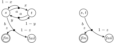
See Fig. 1 for an example of how collapsing EC removes irrelevant distributions.
3.2 Extremal Probability States
Transitions from states with maximal reachability probability 0 or 1 are also irrelevant. Both sets of states can be computed, even if the probabilities are not known, using graph-based algorithms [Courcoubetis and Yannakakis, 1995]. This optimization is also well-known and standard in probabilistic model checking tools. Since, for such states, either a policy exists such that we certainly reach the target set or there is no way to reach the target set of states, clearly transitions leaving them (more precisely, the transitions defined by state-action pairs with them) are irrelevant.
Proposition 2. For all (s, a) ∈ S × A such that Valδ{s↦→1} (T) ∈ {0, 1}, the distribution δ(s, a) is irrelevant.
Collapsing extremal probability states. The above result allows us to assume, without loss of generality, that the MDP has exactly one unique target state fin with maximal reachability probability 1. (If this is not the case, then we redirect all transitions going to those states so that they lead to fin.) Similarly, we can assume there is exactly one state, fail , with maximal reachability probability 0.
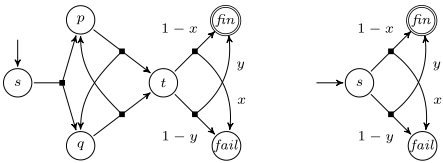
Example 1 (Other irrelevant distributions). Consider the lefthand MDP shown in Fig. 2. Although the transition probabilities for transitions among states s, p, q, t are not given, it is clear that for any policy π, we have P δ,π {s↦→1} [Reach({t})] = 1. In words, t is unavoidable from s, regardless of the probability values that are not shown. Hence, the maximal reachability probability - with respect to s as initial state and fin as target state - only depends on the choice of action from t. Thus, only distributions δ(t, a), for a ∈ A, are not irrelevant, and the MDP can be simplified by transforming it into the right-hand MDP in the figure. Unfortunately the states do not form an EC and, therefore, we cannot obtain the right-hand MDP using the existing reduction rules only.
In the next section we will describe new reduction rules which help, in particular, to achieve the transformation described in the previous example.
4 NewReductions
We now describe new reductions based on a binary relation on the distributions that can be inferred from the directed graph of a given MDP M = (S, A, δ) and target state fin.
4.1 A Preorder on Distributions
For any two state-action pairs (p, a), (q, b) ∈ S × A, we say (q, b) is always (strictly) better than (p, a) if, for all probabilistic transition functions δ′ with supp(δ′ ) = supp(δ),
(resp. <). We then write (p, a) ⊴ (q, b) (resp. ◁) to denote the fact. Given a state-action pair (p, a) and a set P ⊆ S ×A, we lift the relation ⊴ (resp. ◁) to sets by letting (p, a) ⪯ P (resp. ≺) denote the fact that, for all probabilistic transition functions δ′ with the same support as δ, there exists some (q, b) ∈ P such that Equation (1) holds.
Lemma 2. The binary relation ⊴ is a preorder. If (p, a) ≺ P (resp. ⪯) and P ⊆ P ′ , then (p, a) ≺ P ′ (resp. ⪯).
Choosing actions based on the preorder. The main idea behind how we will use the relations ◁,≺ is quite intuitive. If, at a state s, there is a choice of playing actions a, b ∈ A and (s, b) is always better than (s, a), then we remove the possibility of choosing action a. More precisely, if (s, a) ≺ {(s, b) | b ∈ A}, then we can set δ(s′ |s, a) to 0 for all s′ . Regardless of the actual values of the probabilities, any policy maximizing the reachability probability will not play a.
Probability-1 shortcuts. For convenience, in the sequel we assume that for all states s, t ∈ S, if Valδ{s↦→1} ({t}) = 1, then for all (t′ , a) ∈ S ×A with δ(t′ |t, a) > 0 there is some b ∈ A such that δ(t′ |s, b) = δ(t′ |t, a). This assumption is at no loss of generality. If it does not hold, we can apply (in polynomial time) the following pre-processing to the MDP. If from s there is some policy to ensure reaching t with probability 1, then using fresh actions we add shortcuts from s to the distributions δ(t, a) that can be 'chosen' from t.
Example 2. In the left-hand MDP from Fig. 2, we would add shortcuts from s to both distributions available from t. Note that to obtain the desired transformation for this MDP, all that remains is to somehow establish that the newly added shortcuts are always better than the unique state-action pair that was originally available from s (to justify removing the latter).
In what follows we give two sufficient conditions for establishing the 'always better than' relation.
4.2 Sufficient Conditions for the Preorder
Both conditions rely on the notion of separating set.
Separating sets. Consider a set of state-action pairs P ⊆ S ×A. If all runs starting from a state sampled from ι and reaching the state t ∈ S go through some state-action pair from P , we say that P separates t from ι.
Separating sets for fin. Suppose we are given a state-action pair (s, a) ∈ S × A and a set M ⊆ S × A, and we are asked whether (s, a) ⪯ M holds. Denote by P ≺(M) the set of state-action pairs for which there exists some always-better pair in M, i.e. the set {(t, b) ∈ S ×A} | (t, b) ≺ M}. We now claim that if M∪P ≺(M) separates fin from δ(s, a), then (s, a) ⪯ M holds.
Theorem 1. If M ∪P ≺(M) separates fin from δ(s, a), then (s, a) ⪯ M. If additionally, Valδδ(s,a) ({t | ∃b ∈ A : (t, b) ∈ M}) < 1, then (s, a) ≺ M.
Since M ∪ P ≺(M) separates fin from δ(s, a), then for all δ′ with the same support as δ we have that Valδ′ δ′ (s,a) ({fin}) must be equal to a convex combination of the values
{Valδ′ δ′ (t,b) ({fin}) | (t, b) ∈ M ∪ P ≺(M)}. Indeed, by definition of separating sets, any run reaching fin from a state in the support of δ′ (s, a) will first reach a state from {t | (t, b) ∈ (M ∪P ≺(M))}. It is then easy to verify that there exists (t, b) ∈ (M ∪ P ≺(M)) such that Valδ′ δ′ (s,a) ({fin}) ≤ Valδ′ δ′ (t,b) ({fin}), which gives us the first part of the claim. If we also know there is no policy to reach T := {t | (t, b) ∈ M} from δ(s, a) with probability 1, we can then use the definition of P ≺(M) to show that the inequality is strict.
Example 3. Consider again the left-hand MDP from Fig. 2. Recall that we have added shortcuts from s to both distributions available from t (see Ex. 2). Let us denote those two distributions by δ(t, a) and δ(t, b). We can now use Thm. 1 to justify removing the only transition available from s originally. Let us denote the latter by δ(s, a). Clearly, if we remove t from the MDP, then there are no runs which can reach fin from δ(s, a). Hence, {(t, a), (t, b)} separates s from fin. It follows that either (t, a) or (t, b) is always better than (s, a), and that we can remove δ(s, a).
Separating sets for fail. Suppose we are given two stateaction pairs (s, a), (t, b) ∈ S × A and we are asked whether (t, b) ⊴ (s, a) holds. Let P ⊵(t, b) denote the set {(u, c) ∈ S ×A | (t, b) ◁ (u, c)}, and P ▷ (t, b) be defined similarly. We now claim that if there is a policy to reach P ⊵(t, b) ∪ {t, fin} from δ(s, a) with probability 1, then (t, b) ⊴ (s, a) holds.
Theorem 2. · If Valδδ(s,a) ({u | (u, c) ∈ P ⊵(t, b)} ∪ {t, fin}) = 1, then (t, b) ⊴ (s, a).
- If Valδδ(s,a) ({u | (u, c) ∈ P ▷ (t, b)} ∪ {fin}) = 1 also holds, then (t, b) ◁ (s, a).
The intuition why the result holds is as follows. Since there is a policy to ensure reaching {u | (u, c) ∈ P ⊵(t, b)}∪{t, fin} with probability 1, the maximal reachability probability from δ(s, a) must be greater than the least maximal reachability probability from a state in that set. By definition of P ⊵(t, b), all its elements are always better than (t, b). It follows that (s, a) is also always better than (t, b). An alternative way to see it is to notice that {u | (u, c) ∈ P ⊵(t, b)}∪{t, fin} in fact separates fail from δ(s, a) - under some policy. Hence, all runs from δ(s, a) which reach fail pass through the set (which should therefore be avoided if possible).
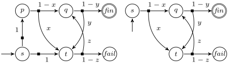
Example 4. Consider the left-hand MDP from Fig. 3. Let us denote by δ(s, a) the distribution assigning probability 1 to state p; by δ(s, b) the one assigning probability 1 to t; by δ(p, a) and δ(t, a) the ones with probability 1 - x and 1 - z of reaching q and fail , respectively. Observe that we have probability-1 shortcuts from s to δ(p, a) and to δ(t, a). All that is left, to obtain the reduced MDP on the right side of the figure, is to argue that (p, a) is always better than the other three pairs so that they can be removed. To do so, we note that from all of them, the only way to reach fail is to go through δ(t, a). The desired relation then holds by Thm. 2.
Algorithm 1 MDP reductions based on irrelevant distributions
1: procedure REDUCE 2: Collapse maximal end components 3: Merge prob. 1 and 0 states 4: Create probability-1 shortcuts 5: alBetter ′ ←∅ 6: repeat 7: alBetter ← alBetter ′ 8: for (s, a) ∈ S × A do 9: M ← {(s, b) | b ̸= a} 10: if isAlwaysBetter(M, (s, a)) then 11: alBetter ′ ← alBetter ′ ∪ {(M, (s, a))} 12: remove (s, a) 13: break // to avoid removing all actions 14: end if 15: end for 16: until alBetter ′ = alBetter 17: end procedure4.3 Summary of the Algorithm
Our proposed reduction algorithm (see Alg. 1) consists in first applying the well-known reductions. Second, create probability-1 shortcuts. Third, for each state s we check whether for some action a, (s, a) is always worse than all alternatives (s, b); if this is the case, then we remove δ(s, a). To determine whether this is the case, we use one of the two conditions described above. More precisely, the isAlwaysBetter function checks the conditions from Thms. 1 and 2 based on the computed relation alBetter -which is initially empty.
Note that the third step is repeated until convergence. The number of iterations before convergence will be linear in the size of the MDP since at least one transition is removed after every iteration.
Recall that after these reductions are applied, the maximal reachability probability in the reduced MDP is equivalent to the maximal reachability probability in the original MDP. Furthermore, both conditions given by Thms. 1 and 2 can be checked in polynomial time. This is because they rely only on deciding whether a given set is a separating set and deciding whether the maximal reachability probability of a distribution is not 0 or 1. Since we repeat the process until convergence, i.e. at most a linear number of times, and the checks in each iteration are computable in polynomial time, the entire procedure takes polynomial time.
5 Experiments
We present some results of running the reduction techniques on two model checking case studies from PRISM [Kwiatkowska et al., 2011], a well-known probabilistic model checking tool, as well as a model-learning task in a gridworld.
| Formula | No reds. | Known reds. | New reds. |
|---|---|---|---|
| ϕ1 | 400 | 392 | 76 |
| ϕ2 | 400 | 392 | 92 |
| Params. | No reds. | Known reds. | New reds. |
|---|---|---|---|
| K = 1 | 553 | 530 | 59 |
| K = 2 | 827 | 804 | 105 |
5.1 Model Checking Experiments
Currently, the most widely used algorithm to model check MDPs in practice is value iteration (see , e.g., [Kwiatkowska et al., 2011; Haddad and Monmege, 2014]). The known upper bound on the number of iterations required for the value obtained to satisfy any formal guarantees is polynomial in the size of the representation of the smallest transition probability of the MDP. This makes reporting running times for value iteration before and after reductions not interesting: in any MDP with irrelevant distributions, we can make the probabilities on those distributions as small as needed to make value iteration (before applying our reductions) take as long as desired.
Randomized Consensus Shared Coin Protocol. We look at a model of an asynchronous shared coin protocol detailed in [Aspnes and Herlihy, 1990]. The goal is to compute the maximal probability of the following two LTL formulas: ϕ1 = ♦("finished" ∧ "all coins equal 1") and ϕ2 = ♦ ("finished" ∧ ¬"all coins equal 1") - where ♦ should be read as eventually. The protocol is modelled in the PRISM language by [Kwiatkowska et al., 2001]. 1 We implement our reduction techniques, as well as the currently-used ones, and the results are given in Tab. 1.
IPv4 Zeroconf Protocol. This problem involves checking for the probability of the host choosing an IP address that is already in use. The corresponding formula is ♦(l = 4 ∧ ip = 1). The protocol is modelled by [Kwiatkowska et al., 2004]. 1 Results of applying the reductions are shown in Tab. 2.
Summary of results. The algorithm results in an 81% and 77% reduction in the size of the randomized consensus MDP compared to the 2% under existing techniques. For the Zeroconf protocol MDP, we were able to achieve 89.3% reduction compared to 4.2% under existing techniques. For both cases, the corresponding LTL formula was verified in the resulting fully reduced MDP. For the randomized consensus and Zeroconf MDPs the maximal probability of satisfying the respective LTL formulas on the reduced MDPs was found to be 0.55, 0.062 and 2.9 × 10⁻⁴ , 5.3 × 10⁻⁵ . This matches the values obtained from PRISM.
1 Model details can be found on the PRISM case studies website. We use model parameters: 2 coins and K = 2, and reset = TRUE and K ∈ {1, 2}, respectively.
| No. states | No reds. | Known reds. | New reds. |
|---|---|---|---|
| 144 | 564 | 273 | 166 |
| 225 | 900 | 423 | 288 |
| 400 | 1600 | 738 | 570 |
5.2 Reductions in Gridworlds with LTLObjective
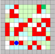
We present an example of a learning problem in a gridworld. For the robot's different actions (heading north ('N'), south ('S'), west ('W') and east ('E')), the probability of arriving at the correct cell is in a certain range: [0.75, 0.80] in this example. With a relatively small probability, the robot will arrive at the cell adjacent to the intended one. For example, with action 'N', the intended cell is the one to the north ('N'), whose the adjacent ones are the northeast ('NE') and northwest cells ('NW'). We look at the specific example shown in Fig. 4.
LTL objective. The objective is to maximize the probability of reaching the green state while avoiding the red ones: ♦R1 ∧□¬R2 where R1 is the green state and R2 is the set of all the red states in the gridworld. The values of the transition probabilities are not known. The underlying task is to learn these probabilities and compute a policy that maximizes the probability of reaching the target. We use a PAC-MDP learning algorithm similar to that shown in [Fu and Topcu, 2014]. In order to mitigate the high sampling requirement and learning time mentioned earlier, we apply the proposed reduction technique to reduce the distributions that need to be sampled without sacrificing the PAC guarantees.
Experiment setup. We test three differently sized gridworlds. For each gridworld we randomly distribute a given number of obstacles, and then apply the reduction techniques. For standardization, 20% of each gridworld was populated with obstacles. Tab. 3 summarizes the average reduction we observe after several runs with a randomized distribution of obstacles in the grid for each run.
Average reduction amount. On average, the size of the fully reduced MDP is about 70% smaller than the original MDP in all three gridworld sizes. The currently applied techniques reduced the size by about 50% in all cases.
| No reds. | Known reds. | New reds. | |
|---|---|---|---|
| Distributions | 400 | 102 | 8 |
| Episodes | 1,133,243 | 948,882 | 83,564 |
| Total steps | 11,683,438 | 7,848,560 | 734,465 |
5.3 Learning in Gridworlds with LTLObjectives
We study the impact of reductions on the learning process.
PAC learning. We now run a modified version of the R-max learning algorithm presented in [Fu and Topcu, 2014] on one of the reduced 10 × 10 MDPs. Explicitly, we aim to learn a policy that with probability at least 1 - δ will be ε-optimal in maximizing reachability probability. We measure the decrease in sampling required before ε-optimality is achieved for ε = 0.01 and δ = 0.05.
Learning results. The number of steps needed for the learning phase is reduced by 94% when the full reductions are implemented compared to 67% under existing techniques.
6 Conclusion and FutureWork
We have proposed a notion of irrelevant distribution to formalize the set of transition probabilities that do not affect the maximal reachability probability. Further, we argue that known MDP reductions, such as collapsing ECs, are in fact removing some irrelevant distributions. We have also described a new algorithm to remove irrelevant distributions which had not, to the best of our knowledge, been considered before. Determining whether our algorithm guarantees that no irrelevant distributions are left, is an open problem.
Our algorithm has been implemented in a prototype tool and empirical results suggest that our algorithm achieves a high reduction rate. Since the results of our experiments show promise, a next step would be to obtain a symbolic version of our algorithm and implement it inside a model-checking tool to determine if the reductions translate into faster running times for model-checking algorithms.
Acknowledgements
This work was supported by the ERC Starting grant 279499 (inVEST) and grants from AFRL #FA8650-15-C-2546, DARPA #W911NF-16-1-0001, and ARO #W911NF-15-1-0592. G. A. P´erez is an F.R.S.-FNRS Aspirant and FWA post-doc fellow.
@inproceedings{ijcai2017p597,
  title     = {Reduction Techniques for Model Checking and Learning in MDPs},
  author    = {Bharadwaj, Suda and Le Roux, Stephane and Perez, Guillermo and Topcu, Ufuk},
  booktitle = {Proceedings of the Twenty-Sixth International Joint Conference on
               Artificial Intelligence, {IJCAI-17}},
  publisher = {International Joint Conferences on Artificial Intelligence Organization},
  editor    = {Carles Sierra},
  pages     = {4273--4279},
  year      = {2017},
  month     = {8},
  note      = {Main track},
  doi       = {10.24963/ijcai.2017/597},
  url       = {https://doi.org/10.24963/ijcai.2017/597},
}
TY - CPAPER TI - Reduction Techniques for Model Checking and Learning in MDPs AU - Bharadwaj, Suda AU - Le Roux, Stephane AU - Perez, Guillermo AU - Topcu, Ufuk T2 - Proceedings of the Twenty-Sixth International Joint Conference on Artificial Intelligence, IJCAI-17 PB - International Joint Conferences on Artificial Intelligence Organization PY - 2017 SP - 4273 EP - 4279 DO - 10.24963/ijcai.2017/597 UR - https://doi.org/10.24963/ijcai.2017/597 ER -Copied
Machine-readable versions of this paper, for tools and AI agents:





