
Efficient Optimal Search under Expensive Edge Cost Computation
Proceedings of the Twenty-Sixth International Joint Conference on Artificial Intelligence. Main track. Pages 4266-4272.
https://doi.org/10.24963/ijcai.2017/596
Keywords
- Planning and Scheduling: Search in Planning and Scheduling
- Combinatorial & Heuristic Search: Heuristic Search
Abstract
Optimal heuristic search has been successful in many domains, including journey planning, route planning and puzzle solving. Existing work typically assumes that the cost of each action can easily be obtained. However, in many problems, the exact edge cost is expensive to compute. Existing search algorithms face a significant performance bottleneck, due to an excessive overhead associated with dynamically calculating exact edge costs.
We present DEA*, an algorithm for problems with expensive edge cost computations. DEA* combines heuristic edge cost evaluations with delayed node expansions, reducing the number of exact edge computations. We formally prove that DEA* is optimal and it is efficient with respect to the number of exact edge cost computations.
We empirically evaluate DEA* on multiple-worker routing problems where the exact edge cost is calculated by invoking an external multi-modal journey planning engine. The results demonstrate the effectiveness of our ideas in reducing the computational time and improving the solving ability. In addition, we show the advantages of DEA* in domain-independent planning, where we simulate that accurate edge costs are expensive to compute.
- [Amir and Engelhardt, 2003] Eyal Amir and Barbara Engel- hardt. Factored Planning. In Proceedings of the International Joint Conference on Artificial Intelligence (IJCAI), 2003.
- [Asai and Fukunaga, 2015] Masataro Asai and Alex Fukunaga. Solving Large-Scale Planning Problems by Decomposition and Macro Generation. In Proceedings of the International Conference on Automated Planning and Scheduling(ICAPS), Jerusalem, Israel, June 2015.
- [Asai and Fukunaga, 2016] Masataro Asai and Alex Fukunaga. Tiebreaking Strategies for Classical Planning Using A * Search. In Proceedings of the AAAI Conference on Artificial Intelligence, Arizona, USA, February 2016.
- [Botea and Braghin, 2015] Adi Botea and Stefano Braghin. Contingent versus Deterministic Plans in Multi-Modal Jour- ney Planning. In Proceedings of the International Conference on Automated Planning and Scheduling(ICAPS), volume 15, pages 268-272, 2015.
- [Botea et al., 2013] Adi Botea, Evdokia Nikolova, and Michele Berlingerio. Multi-Modal Journey Planning in the Presence of Uncertainty. In Proceedings of the International Conference on Automated Planning and Scheduling(ICAPS), 2013.
- [Brafman and Domshlak, 2006] Ronen I Brafman and Carmel Domshlak. Factored Planning: How, When, and When Not. In Proceedings of the AAAI Conference on Artificial Intelli- gence, 2006.
- [Du and Leung, 1990] Jianzhong Du and Joseph Y-T Leung. Minimizing Total Tardiness on One Machine is NP-Hard. Mathematics of Operations Research, 15:483-495, 1990.
- [Goldenberg et al., 2014] Meir Goldenberg, Ariel Felner, Roni Stern, Guni Sharon, Nathan R Sturtevant, Robert C Holte, and Jonathan Schaeffer. Enhanced Partial Expansion A*. J. Artif. Intell. Res.(JAIR), 50:141-187, 2014.
- [Hart et al., 1968] Peter E. Hart, Nils J. Nilsson, and Bertram Raphael. A Formal Basis for the Heuristic Determination of Minimum Cost Paths. Systems Science and Cybernetics, IEEE Transactions on, 4(2):100-107, 1968.
- [Haslum and Geffner, 2000] Patrik Haslum and Héctor Geffner. Admissible Heuristics for Optimal Planning. In Proceedings of the International Conference of AI Planning Systems, 2000.
- [Helmert and Domshlak, 2009] Malte Helmert and Carmel Domshlak. Landmarks, Critical Paths and Abstractions: What's the Difference Anyway? In Proceedings of the In- ternational Conference on Automated Planning and Schedul- ing(ICAPS), 2009.
- [Helmert and Röger, 2008] Malte Helmert and Gabriele Röger. How Good is Almost Perfect? In Proceedings of the AAAI Conference on Artificial Intelligence, 2008.
- [Helmert, 2006] Malte Helmert. The Fast Downward Planning System. J. Artif. Intell. Res.(JAIR), 26:191-246, 2006.
- [Kishimoto and Nagano, 2016] Akihiro Kishimoto and Kiy- ohito Nagano. Evaluation of Auction-Based Multi-Robot Routing by Parallel Simulation. In Proceedings of the In- ternational Conference on Automated Planning and Schedul- ing(ICAPS), pages 495-503, 2016.
- [Kishimoto and Sturtevant, 2008] Akihiro Kishimoto and Nathan Sturtevant. Optimized Algorithms for Multi-Agent Routing. In Proceedings of the International Conference on Autonomous Agents and Multi-Agent Systems, pages 1585-1588, 2008.
- [Kishimoto et al., 2016] Akihiro Kishimoto, Adi Botea, and Elizabeth Daly. Combining Deterministic and Nondetermin- istic Search for Optimal Journey Planning Under Uncertainty. In Proceedings of the European Conference on Artificial In- telligence, volume 285, page 295. IOS Press, 2016.
- [Korf, 1985] Richard E. Korf. Depth-First Iterative-Deepening: An Optimal Admissible Tree Search. Artificial Intelligence, 27(1):97-109, 1985.
- [Phillips et al., 2014] Mike Phillips, Maxim Likhachev, and Sven Koenig. PA* SE: Parallel A* for Slow Expansions. In Proceedings of the International Conference on Automated Planning and Scheduling(ICAPS), 2014.
- [Richter and Helmert, 2009] Silvia Richter and Malte Helmert. Preferred Operators and Deferred Evaluation in Satisficing Planning. In Proceedings of the International Conference on Automated Planning and Scheduling(ICAPS), pages 273- 280, 2009.
- [Sturtevant et al., 2015] Nathan R. Sturtevant, Jason M. Traish, James R. Tulip, Tansel Uras, Sven Koenig, Ben Strasser, Adi Botea, Daniel Harabor, and Steve Rabin. The Grid-Based Path Planning Competition: 2014 Entries and Results. In Pro- ceedings of the Annual Symposium on Combinatorial Search, pages 241-251, 2015.
- [Tolpin et al., 2013] David Tolpin, Tal Beja, Solomon Eyal Shi- mony, Ariel Felner, and Erez Karpas. Towards rational de- ployment of multiple heuristics in A*. In Proceedings of the International Joint Conference on Artificial Intelligence (IJ- CAI), pages 674-680, 2013.
- [Yoshizumi et al., 2000] Takayuki Yoshizumi, Teruhisa Miura, and Toru Ishida. A* with Partial Expansion for Large Branch- ing Factor Problems. In Proceedings of the AAAI Conference on Artificial Intelligence, pages 923-929, 2000.
References were extracted automatically from the PDF and may contain errors.
Full text extracted automatically from the PDF; figures, tables and equations may differ. The PDF is the version of record.
1 Introduction
Heuristic search can tackle many difficult problems, including puzzles, journey planning and route planning e.g., [Korf, 1985; Botea et al., 2013; Sturtevant et al., 2015]. Algorithms such as A* [Hart et al., 1968] can be used to find optimal solutions. Existing optimal heuristic search algorithms typically assume that edge costs are known a priori. For example, the unit edge cost of 1 is used to find the smallest number of moves to solve a sliding puzzle instance. In the Traveling Salesperson Problem (TSP), the cost of an edge is typically fixed, and edge costs are obtained with a negligible computational overhead (e.g., using table lookups).
However, in some domains, it is difficult to pre-compute the exact edge costs. They must be computed dynamically, during search. When dynamic edge cost computations are expensive, optimal heuristic search faces a major challenge stemming from an excessive overhead caused by edge cost computations.
∗This work was performed in IBM Research, Ireland. He is also supported by a JSPS Grant-in-Aid.
Consider the TSP in a setting where a city's multi-modal transport network is used for travel. The travel time between two locations can depend on factors such as the departure time and uncertain events such as traffic jams. Multi-modal journey planning can provide travel times between two locations, with a given starting time, taking into account uncertainty, such as potential missed connections due to variations in the arrival and departure bus times [Botea et al., 2013].
Despite recent advances in optimal multi-modal journey planning under uncertainty [Botea and Braghin, 2015; Kishimoto et al., 2016], computing the optimal travel time can be expensive. For instance, Kishimoto et al. (2016) showed cases where their journey planner needs 100 seconds and visits 1 million nodes to compute one journey plan between two locations for a given departure time. In addition, the optimal travel time between two locations cannot be precomputed and stored in a table due to prohibitively many combinations of an origin, a destination, and a departure time.
We present Delayed Expansion A* (DEA*), an A* variant that performs efficient, dynamic edge cost computations, during heuristic search. With admissible estimates of exact edge costs, DEA* can delay the computation of exact edge costs. This way, DEA* reduces the number of exact edge computations while always producing optimal solutions. Besides the main DEA* algorithm, we describe several search enhancements such as dominance-based pruning, and caching.
Part of the evaluation focuses on a problem called Multiple-Worker Routing Problem (MWRP). We introduce MWRP and prove that MWRP is an NP-hard problem. Besides MWRP, we demonstrate our ideas in domainindependent planning problems, where we simulate that exact edge costs might be expensive to compute. Our results clearly show that our approach significantly reduces the computational time and improves the solving ability.
2 Delayed Expansion A*
In this section, we present our algorithm DEA*. Consider a problem P where edge costs are expensive to compute. As said earlier, examples could include edges representing a travel leg, from an origin to a destination, in a multi-modal travel network characterized by uncertainty. If A* is used to
Algorithm 1 DEA*
Input: n0 1: Initialize OPEN← ∅, g(n0) ← 0, (∀n ̸= n0; g(n) ←∞) 2: insert(n0,OPEN), Mark s0 as standard (i.e., not temporary) 3: while OPEN ̸= ∅ do 4: n← deleteMin(OPEN) 5: if n has a duplicate n′ ∈ CLOSED and g(n′ ) ≤ g(n) then 6: Continue 7: else if n is temporary then 8: g(n) ← g(parent(n)) + ca(parent(n), n) 9: Adjust s(n), h(n), f(n) based on ca 10: insert(n, OPEN), Mark n as standard (i.e., not temporary) 11: Continue 12: else 13: Add n to CLOSED, Update g(n) in CLOSED if better g-value is found 14: if n is a goal then 15: Extract and return solution 16: Generate successors(n) based on ch 17: for each m ∈ successors(n) do 18: gh ← g(n) + ch(n, m) 19: g(m) ← gh, parent(m) ← n 20: insert(m, OPEN), Mark m as temporarysolve such a problem P, every time when A* traverses 1 an edge in the search graph, the exact cost of that edge has to be available. A* could compute these costs on demand, and cache the results for a future reuse.
However, caching and reusing actual costs have a limited usefulness. At the same time, heuristic admissible estimations for travel times can often be provided much more quickly. DEA* takes advantage of this, using heuristic estimates of edge costs to delay or even avoid entirely the computation of an accurate cost. Often, an optimal solution is found with no need to compute accurate costs for all generated nodes. This is where the advantage of DEA* stems from.
In the rest of this section we describe DEA*, provide an example and perform a theoretical analysis of DEA*.
2.1 The DEA* Algorithm
Given a search node n, assume that n contains state information s(n), a pointer to the parent node, a g-value g(n) that is the sum of the edge costs from the initial state to n, a h-value h(n) that is a heuristic estimation of the cost from n to reach a goal, and a function f = g + h. DEA*'s heuristic function is admissible, never overestimating the optimal cost to reach a goal, and thus ensuring solution optimality. In DEA*, we distinguish between two types of edge costs, namely an admissible heuristic estimation ch and an actual cost ca.
Consider an edge (p, n) from a parent node to a successor node. Using a heuristic cost for this edge could impact g(n), s(n), h(n) and f(n), as follows. By definition, g is impacted, as g is the sum of all edge costs of the path available from the root to n. To show the potential impact on s(n), consider a problem where some edges encode traveling legs from one location to another. Assume further that the arrival time at a current location is part of the state definition. Clearly, the arrival time can depend on the cost of the incoming edge, i.e., on the travel time from a previous location to the current location. The heuristic h(n) could be impacted because it typically is a function of the state information s(n).
1 We say that A* traverses an edge if that edge is the transition from a node currently being expanded to a successor.
Algorithm 1 shows DEA* in pseudocode built on top of A*. For clarity, the pseudocode is based on a simple variant of A*. A newly generated node n could be discarded straight away if a duplicate n′ exists in CLOSED with f(n′ ) < f(n). The pseudocode does not show this, for simplicity.
In DEA*, when a node p is expanded (and thus a successor n is generated), only the heuristic cost ch of the edge (p, n) is computed. Node data such as g(n), s(n), h(n), f (n) are computed with the heuristic cost ch in use for the edge (p, n).
After being generated, n is enqueued into the OPEN list based on the heuristic cost ch. A node enqueued into the OPEN in this fashion is called a temporary node. When a temporary node n is popped from OPEN, the actual cost ca of the edge from its parent is computed, and g(n), s(n), h(n) and f(n) are updated accordingly. The node changes its status from a temporary node into a standard node. The node is re-inserted into the OPEN list with the new f value, and the main cycle of DEA* continues.
2.2 Example
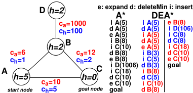
Fig. 1 illustrates differences between DEA* and A* on a toy, 4-node search graph. A* expands the nodes A, B and C in this order, during which it evaluates the actual cost of edges AB, AC, BD and BC in this order. The computation of BD, which yields a value of 1000, is unnecessary, since all other edge costs are significantly smaller.
DEA* does not compute the actual cost ca of edge BD. After the root node A is expanded, B and C are enqueued with f values based on ch estimations of the edges from their parent. Then B, whose f value is 3, is popped from the OPEN list. Now the actual cost ca of the edge AB is computed, and f(B) becomes 6 + 2 = 8. In this simple example, we assume that the h value of a node stays constant (i.e, it does not change when a node changes its status from temporary to permanent). Node B is re-inserted into the OPEN, and node C is popped out. Its f value increases from 5 to 10, which triggers its re-insertion into the OPEN, with the new f value. The process continues as shown in Fig. 1, with node D never being popped from the OPEN.
As illustrated in Fig. 1, DEA* can perform more OPEN list operations than standard A*. However, in scenarios where edge cost computations, or even state heuristic computations are expensive, OPEN list operations have a much smaller impact on the overall running time.
2.3 Theoretical Analysis
We prove two theoretical properties of DEA*.
Theorem 1. DEA* outputs optimal solutions.
Proof sketch. DEA* expands only regular nodes, i.e., nodes computed with ca in use. Given DEA*, consider an underlying A* that breaks ties among nodes in the OPEN in the same way as DEA*. DEA* and the A* under consideration expand the same set of nodes, in the same order.
Based on the two facts above, it follows that DEA* and the corresponding A* compute identical solutions. □
Given a node n, let nh be its temporary version, and na its standard version. Let p be the parent node. Note that p is already a standard node at the time when n is generated, since nodes are expanded only after they become standard nodes. Define g(na) = g(p) + ca(p, na), and g(nh) = g(p) + ch(p, nh). We say that the heuristic h is consistent with respect to ch if, for every parent-child pair (p, n), h(p) ≤ ch(p, nh) +h(nh) and h(G) = 0 for every goal node G. Assuming further that h(nh) ≤ h(na), ∀n, if h is consistent with respect to ch, it is also consistent with respect to ca (i.e., standard consistency).
Theorem 2. Assume that A* and DEA* use a similar tie breaking scheme, and that they use a heuristic h that is consistent with respect to ch. DEA* cannot generate more nodes with actual edge costs than A*.
Proof. Let c∗ be the optimal cost of a solution. The set of nodes that DEA* generates using ca includes the set S1 of all nodes n with f(nh) < c∗ , plus S2, a subset of the nodes n with f(nh) = c∗ , depending on tie breaking. The set of nodes generated by A* includes the set S3 of all nodes n with f(parent(n)) < c∗ , plus S4, a subset of all nodes n with f(parent(n)) = c∗ , depending on tie breaking.
Let n be a node and let p be its parent. Then f(p) = g(p)+ h(p) ≤ g(p) + ch(p, nh) + h(nh) = f (nh).
It follows that S1 ⊆ S3 and S2 ⊆ S4, assuming a similar tie-breaking scheme. □
3 The Multiple-Worker Routing Problem
MWRP is a realistic scheduling problem that requires finding an optimal schedule for a set of workers to deliver services to a set of customers residing at different fixed locations. For simplicity and without loss of generality, we consider a simple healthcare scenario where the customers are patients and the workers deliver at-home care services such as nursing care, medical care, and physical therapy. Each patient has an appointment time when a worker should arrive and perform a healthcare task. To visit and treat patients, a worker uses the multi-modal public transport available in a city. Emergency situations, where using an ambulance is more appropriate, are beyond our focus. So is the rescheduling and the dynamic assignment or reassignment of tasks.
In a valid solution, all patients have to be treated. Tasks can be performed later than their appointment time, but each delay in performing a task degrades the quality of a solution. The cost of a solution is the sum of all delays of all tasks.
A task starting at its planned appointment time has no delay (i.e., the delay is 0). Tasks starting later have a positive delay. A task cannot start earlier than their planned appointment time (i.e., even if the worker arrives early, they will have to wait until the task is supposed to start).
For simplicity, the duration of each treatment is set to 0. Setting a deterministic task duration in MWRP does not change MWRP's computational difficulty. Considering nondeterministic treatment duration remains future work.
More formally, a four-tuple 〈P, A, W, τ (x, y, t)〉 defines an MWRP, where P = {pi|1 ≤ i ≤ n} is a list of locations of the patients, A = {ai|1 ≤ i ≤ n} is a list of appointment times, W = {wj|1 ≤ i ≤m} is a list of initial locations of workers and τ(x, y, t) is a travel time function between two locations x, y ∈ P ∪W with the start time t ∈ [0, 86400]. 2
It is important to note that in practice the travel time depends on the start time, the schedules of the public transport vehicles, and the other factors such as uncertainty about the actual arrival and departure times of buses.
We show that solving MWRP optimally is NP-hard. We define the MWRP-OPT problem as follows. The input is an MWRP instance and a number k ≥ 0. The question is whether the instance has a solution whose cost (delay) D satisfies D ≤ k.
Theorem 3. MWRP-OPT is NP-hard.
Proof. We show this with a reduction from the single machine total tardiness problem (SMTTP), an NP-hard problem [Du and Leung, 1990]. Given a set of jobs {1, 2, · · · , n} to be processed on a single machine and the processing time pti and due date di of each job i, the objective is to find a schedule for the jobs that minimizes the tardiness T = ∑ni=1 Ti, where Ti = max(0,Ci - di) and Ci is the completion time of job i according to the schedule.
Consider an arbitrary SMTTP instance defined as above. We construct an MWRP instance in polynomial time as follows. There is one worker and n patients. The appointment time of patient i is di, and the duration of the appointment (treatment) is 0. The worker walks between locations, and the travel time from location j (j ̸= i) to location i is pti.
It is easy to see that the tardiness T in the SMTTP instance is equal to the total delay (i.e., the cost) D of the MWRP instance. Thus, the SMTTP instance has a solution with T ≤ k iff the MWRP instance has a solution with D ≤ k. □
State Space Representation
We next define the state space used for solving MWRP. A search state is represented by 3-tuple 〈B, T, L〉 where B = {bi|1 ≤ i ≤ n} is a bit vector representing whether a patient i has already been treated, T = {tj|1 ≤ j ≤m} is a list of current times of the workers and L = {li|1 ≤ i ≤ m} is a list of locations of workers at time tj.
We define a single action schema, denoted by treat(i, j), where i is a patient and j is a worker. A treat action has the following effects. The bit bi corresponding to patient i is set to true. The current time tj of worker j is updated as follows. As tasks do not start before the appointment time ai, the worker's time is set to either the arrival time, or the appointment time, whichever comes later: tj ← max(tj + τ(lj, pi, tj), ai). Finally, the location lj of worker j is updated to the location pi of the patient i.
2 86400 = 24 × 60 × 60 is the number of seconds in a day.
The cost of an action is defined by the delay, namely max(tj + τ(lj, pi, tj) - ai, 0). This means that the delay is 0 when the worker arrives in time or earlier than the appointment time. Otherwise, the delay is positive.
A solution to an MWRP instance M is a sequence of actions treat(i, j) where every appointment is addressed with a treat action. The solution cost is the sum of the action delays. An optimal solution minimizes the total delay.
In this MWRP setting, the travel time between two locations (i.e., τ(·)) is not given a priori. In practice, the actual travel time depends on multiple factors such as the origin, the destination, the time of travel, and the uncertainty about the multi-modal transportation network (e.g., exact arrival and departure times for buses). Pre-computing accurate values for all travel times often is impractical, due to many combinations of origins, destinations, and departure times.
4 Search Enhancements inMWRP
We present a pruning strategy based on state dominance, an admissible heuristic h, and other implementation details.
State dominance
We assume the following monotonicity over the arrival time of a trip:
Assumption 1. For any start time t1 ≤ t2, it holds that t1 + τ (x, y, t1) ≤ t2 + τ (x, y, t2).
This implies the following property:
Proposition 1. The delay d(i, j) = max(tj + τ(lj, pi, tj) - ai, 0) is monotonically increasing over tj .
Given that the cost of a path is a sum of delays, we get the following dominance criterion:
Definition 1. For two states s1 and s2, we say that s1 dominates s2 (denoted as s1 ≤ s2) when ∀j, tj(s1) ≤ tj(s2) and ∀j, lj(s1) = lj(s2) and ∀i, bi(s1) = bi(s2).
For such states, the cost of an optimal path containing s1 is no greater than the cost of an optimal path containing s2. Thus it is safe to prune dominated states without losing the optimality of the solution computed.
Note that DEA* does not apply the dominance relationship when the dominating node is a temporary node. This is because the current time of the temporary node could be updated to a larger value when the node is reevaluated (i.e., when the node is converted into a standard node).
Admissible heuristic
We have implemented a variant of the h2 heuristic [Haslum and Geffner, 2000], adapted to MWRP. Since the computation of h2 requires the edge costs of all applicable actions available at the current state, a straightforward implementation results in extensive computations of accurate travel costs. We address this bottleneck by using heuristic cost ch. That is, the computation of the h2 heuristic uses heuristic estimations of travel times, instead of accurate travel times.
In our implementation, both accurate travel times and heuristic travel times are obtained with the DIJA journey planning system [Botea et al., 2013]. The heuristic estimations are computationally cheaper than the actual travel times. The results of invoking DIJA, both for heuristic and actual times, are cached for a future reuse.
DIJA pre-computes a lookup table of admissible heuristic estimates of travel times [Botea et al., 2013]. The system can combine deterministic and non-deterministic search [Kishimoto et al., 2016]. Specifically, it can run a deterministic A* that computes the travel time for an optimistic, best-case scenario (e.g. buses arrive in time). Deterministically computed travel times can be used as an admissible heuristic for an AO* search that computes an uncertainty-aware, contingent plan. We use the search result of DIJA's A* to compute heuristic travel times (ch). We denote this heuristic travel time by τ ′ (x, y, t). The function τ ′ also satisfies the admissibility and monotonicity criteria that hold for τ in Proposition 1.
The h2 heuristic is computed as follows: For each of every combinations of two subgoals (treating the corresponding patients), compute the minimum cost sum (the sum of delays) for achieving them, and return their maximum. The cost is calculated based on ch. Since ch ≤ ca, a h2 heuristic calculated with ch is a lower bound for a h2 heuristic calculated with ca, which is in turn a lower bound of the total cost from the current state to a goal state. Thus, the h2 heuristic computed with ch is admissible.
As mentioned in Sec. 2, amending the cost of the edge from the parent can impact the state, which contains the current time of each worker. This change in the state can also trigger a change in the heuristic value of that node. Thus, heuristic functions might have to be computed twice for a node: once when the node is temporary, and once after the node becomes a standard node.
We can further enhance DEA* with a combination of the hmax (aka the h1 heuristic) and h2 heuristics. Temporary nodes are evaluated with h1 , and standard nodes with h2 . We chose this enhancement because it can be trivially implemented in DEA*. In contrast, A* needs a significant modification to the algorithm in order to adopt this approach.
Finally, A*'s performance is often affected by the tiebreaking strategy [Asai and Fukunaga, 2016]. Ties on the f value are broken by preferring states with fewer untreated patients, and further ties are broken in the first-in-last-out order.
Other implementation details
DIJA's AO* search produces an optimal contingent plan. In a DIJA optimal contingent plan, there is one safe pathway, and zero or more opportunistic pathways. All actions along the safe pathway can be executed with a probability of 1, if the traveler decides to follow that pathway. The safe pathway is the slowest (i.e., has the largest travel time) among all pathways in the optimal contingent plan. Opportunistic pathways are faster, but there is no guarantee that the traveler will be able to follow them at the plan execution time.
For the actual edge cost function ca we currently use the travel time of the safe pathway. Other options for implementing ca, such as using the expected arrival time, are left as future work. However, even with the current actual edge cost function, thanks to the opportunistic pathways, workers have a chance of reducing their delays in practice.
| city | nodes | segments | stops | routes | trips/day |
|---|---|---|---|---|---|
| Dublin | 301,638 | 319,846 | 4,739 | 120 | 7,308 |
| Montpellier | 152,949 | 161,768 | 1,297 | 36 | 3,988 |
| Rome | 522,529 | 566,400 | 8,896 | 391 | 39,422 |
| City | Blind | hmax | h2 | h1h2 | ||||
|---|---|---|---|---|---|---|---|---|
| |W| | A* | DEA* | A* | DEA* | A* | DEA* | DEA* | |
| Total | 50 | 59 | 68 | 77 | 81 | 83 | 85 | |
| Dublin | 12 | 14 | 15 | 15 | 21 | 19 | 22 | 22 |
| 6 | 2 | 4 | 8 | 8 | 12 | 12 | 11 | |
| Montpellier | 12 | 16 | 15 | 17 | 17 | 17 | 15 | 18 |
| 6 | 1 | 4 | 3 | 5 | 3 | 4 | 5 | |
| Rome | 12 | 15 | 18 | 18 | 19 | 19 | 19 | 20 |
| 6 | 2 | 3 | 7 | 7 | 11 | 11 | 9 | |
5 Experimental Results
We evaluate DEA*'s performance in the MWRP and in domain-independent planning. Experiments are conducted on an Intel Xeon CPU cluster, with a time and memory limit of one hour and 1.5 million in-memory states per instance.
Evaluation in the MWRP
We generated a total of 180 instances with the real road-map and transportation data from three European cities (Table 1). In each instance, there are either 6 or 12 workers, while the number of patients was varied between 8-24. They do not contain unrealistic configurations (e.g. 6 workers & 24 patients means that each worker attends 4 patients per hour on average). The map roughly contains an area within a radius of 10km, 6km, and 10km from the city center in Dublin, Montpellier and Rome, respectively. In these maps, the locations of workers W and the locations of patients P are randomly selected within a 2km radius circle in the city center. Appointment times are randomly set between 10-11AM. Workers' start times are fixed at 10AM.
Our evaluation includes three heuristics used in DEA*: blind, hmax (aka h1 ), and h2 . Compared to h2 , hmax is faster but less informative, since it returns only the maximum of the minimum possible delay for each untreated patient. Table 2 shows the number of instances solved by A* and DEA*. In terms of total coverage, DEA* always solves more instances than A*, when they both use the same heuristic. That is, a blind DEA* solves 9 more instances than a blind A*, DEA* with h1 solves 9 more instances than A* with h1 , and DEA* with h2 solves 2 extra instances as compared to A* with h2 .
Moreover, the combined use of h1 and h2 enables DEA* to solve two additional instances compared to DEA* (h2 ), achieving the best solving ability (see h1h2 in Table 2). The results clearly show the importance of our delayed node evaluation in the presence of expensive edge cost computations.
DEA*'s OPEN list is typically twice as large as that of A*. If the edge costs are not too expensive to compute, the OPEN list overhead outweighs the gains resulted from the delayed edge computation, resulting in A* solving two more instances than DEA* in Montpellier with h2 in use.
External Runtime using A*
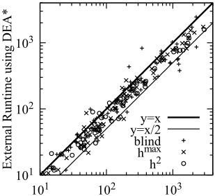
Figure 3: Comparison of the runtime spent for the external calls to DIJA on instances solved by both A* and DEA*
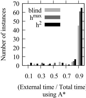
The histogram shown in Fig. 2 indicates the ratio of the runtime spent by the external DIJA engine to the total time of A* + DIJA. Despite integrating caching, the edge cost computations are the main performance bottleneck in A*. In most cases, irrespective of the heuristics used, calls to DIJA cover more than 90% of the runtime of A* + DIJA.
Fig. 3 plots the runtime spent on the external calls to DIJA, for the instances solved by both DEA* and A*. The time spent by A* is plotted on the horizontal axis against DEA* on the vertical axis on logarithmic scales. Points below the y = x line indicate that DEA* outperforms A*. These figures clearly show that DEA* successfully reduces the number of expensive calls to DIJA. The average improvement to the total runtime was 54% (blind), 123% (hmax ), and 149% (h2 ).
Note that these two charts do not show the best performing version of DEA*, namely DEA* with h1h2 . The reason is that in these charts we wanted to compare DEA* vs A* when both algorithms use the same heuristic.
Evaluation in Domain Independent Planning
We consider the case where domain independent classical planning needs to account for the expensive edge cost evaluation. Current domain independent planners support the cases Number of exact edge computations for A*
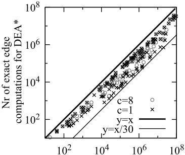
Figure 4: DEA* vs A* in domain independent planning.
where the exact edge costs are obtained easily. For this reason, we simulate that accurate edge costs might be computationally expensive to obtain, and that a cheaper heuristic estimation can be computed.
We implemented DEA* on top of the cost-optimal Fast Downward planner based on the landmark-cut heuristic [Helmert and Domshlak, 2009]. We selected domains with non-unit action costs from the optimal tracks in past International Planning Competitions. We then assumed that Fast Downward can obtain the heuristic edge cost ch by subtracting a constant c from the actual edge cost ca, i.e. ch = max(0, ca - c), as inspired from [Helmert and R¨oger, 2008].
We selected the following non-unit action cost domains: barman, cybersec, elevators, floortile, openstacks, parcprinter, pegsol, scanalyzer, sokoban, transport and woodworking, and considered 20 instances in each domain. We ran the solver with a time and memory limit of 30 minutes and 4GB per instance. hLMcut is computed based on ch, similarly to the heuristics h1 and h2 implemented in MWRP.
In Fig. 4, the number of ca (i.e., exact edge) calculations of A* for each instance is plotted on x-axis, against DEA* on y-axis, on logarithmic scales. We show results obtained with c = 8 and c = 1, and DEA* significantly reduces the number of exact edge cost computations. In terms of the improvement factor (i.e. x/y), when c = 8, the minimum factor is 1.6, the mean 4.5 and the maximum 18. For c = 1, the improvements are even greater. The minimum improvement factor is 1.7, the mean factor is 6.5 and the maximum one is 29.
6 RelatedWork
DEA* is related to Partial Expansion A* (PEA*) [Yoshizumi et al., 2000] and Enhanced PEA* (EPEA*) [Goldenberg et al., 2014]. However, these aim at different types of improvements. PEA* addresses high memory requirements caused by a large branching factor. For example, in the Multiple Sequence Alignment (MSA), the flagship application domain of PEA*, the number of successors per state is O(2d ) where d is the number of sequences to be aligned. PEA* generates and evaluates all successors of a search state but keeps in memory only a partial subset of successors that look promising. As PEA* evaluates every successor, it requires that exact edge costs are immediately available and thus node evaluations are relatively cheap. On the other hand, DEA* addresses the issue of expensive exact edge cost computations required for obtaining the g-value. When a node n is generated, DEA* uses a heuristic estimation of the cost of the edge from its parent. The exact cost computation of that edge is delayed until n is selected for expansion.
Lazy A* [Tolpin et al., 2013] improves and updates the heuristic value. Although Lazy A* is similar in spirit to DEA*, our focus is not on the node estimate, but on the edge cost estimate which requires expensive computations.
Phillips et al. (2014) present PA*SE, a parallel A* for robot motion planning domains. PA*SE is designed for domains where generating successor states can be expensive. E.g., in motion planning problems successor generation may involve an expensive and precise collision checking procedure. In contrast, DEA* is designed for domains where generating successors is not expensive, but computing the exact cost of a parent-successor edge could be.
Deferred evaluation (DE) has been studied in satisficing domain independent planning [Helmert, 2006; Richter and Helmert, 2009]. When generating a successor of a node, DE sets the heuristic value of the successor to that of the parent, thus deferring the successor evaluation. As opposed to DEA*, this related work assumes that edge costs are readily available, and suboptimal solutions are allowed.
Decentralized, auction-based multi-agent coordination has been studied in multi-robot routing problems [Kishimoto and Sturtevant, 2008; Kishimoto and Nagano, 2016]. Edge costs are dynamically computed via path-finding on road or game maps. The similarity to DEA* is that edge costs can be expensive to compute. A key difference is that auction-based techniques are suboptimal.
7 Conclusions
Heuristic search algorithms typically assume that the cost of edges in the search graph are readily available. However, in real-life domains, such as problems that involve traveling between various locations on a map, such a simplifying assumption does not always hold.
We have introduced DEA*, capable to reduce the number of exact edge cost computations. We formally introduced the Multiple Worker Routing Problem, a practical application domain inspired from the healthcare industry. We provided an NP-hardness result for MWRP. We evaluated the performance of DEA* in MWRP and in domain-independent planning. The results demonstrate a significant performance improvement of DEA* as compared to A*.
As future work, Factored Planning [Amir and Engelhardt, 2003; Brafman and Domshlak, 2006; Asai and Fukunaga, 2015] could incorporate ideas from DEA*. This framework automatically decomposes the input problem and solves each subproblem to convert the subplans into macro actions. DEA* could improve this potential bottleneck by replacing the subproblem solving with a partial computation of the plan.
@inproceedings{ijcai2017p596,
  title     = {Efficient Optimal Search under Expensive Edge Cost Computation},
  author    = {Asai, Masataro and Kishimoto, Akihiro and Botea, Adi and Marinescu, Radu and Daly, Elizabeth M. and Kotoulas, Spyros},
  booktitle = {Proceedings of the Twenty-Sixth International Joint Conference on
               Artificial Intelligence, {IJCAI-17}},
  publisher = {International Joint Conferences on Artificial Intelligence Organization},
  editor    = {Carles Sierra},
  pages     = {4266--4272},
  year      = {2017},
  month     = {8},
  note      = {Main track},
  doi       = {10.24963/ijcai.2017/596},
  url       = {https://doi.org/10.24963/ijcai.2017/596},
}
TY - CPAPER TI - Efficient Optimal Search under Expensive Edge Cost Computation AU - Asai, Masataro AU - Kishimoto, Akihiro AU - Botea, Adi AU - Marinescu, Radu AU - Daly, Elizabeth M. AU - Kotoulas, Spyros T2 - Proceedings of the Twenty-Sixth International Joint Conference on Artificial Intelligence, IJCAI-17 PB - International Joint Conferences on Artificial Intelligence Organization PY - 2017 SP - 4266 EP - 4272 DO - 10.24963/ijcai.2017/596 UR - https://doi.org/10.24963/ijcai.2017/596 ER -Copied
Machine-readable versions of this paper, for tools and AI agents:





