
Understanding and Exploiting Language Diversity
Proceedings of the Twenty-Sixth International Joint Conference on Artificial Intelligence. Main track. Pages 4009-4017.
https://doi.org/10.24963/ijcai.2017/560
Keywords
- Natural Language Processing: Natural Language Semantics
- Multidisciplinary Topics and Applications: Multidisciplinary Topics and Applications
- Natural Language Processing: Resources and Evaluation
Abstract
The main goal of this paper is to describe a general approach to the problem of understanding linguistic phenomena, as they appear in lexical semantics, through the analysis of large scale resources, while exploiting these results to improve the quality of the resources themselves. The main contributions are: the approach itself, a formal quantitative measure of language diversity; a set of formal quantitative measures of resource incompleteness and a large scale resource, called the Universal Knowledge Core (UKC) built following the methodology proposed. As a concrete example of an application, we provide an algorithm for distinguishing polysemes from homonyms, as stored in the UKC.
- [Apresjan, 1974] Ju D Apresjan. Regular polysemy. Linguis- tics, 12(142):5-32, 1974.
- [Aronoff and Rees-Miller, 2003] Mark Aronoff and Janie Rees-Miller. The handbook of linguistics, volume 43. John Wiley & Sons, 2003.
- [Bell, 1978] Alan Bell. Language samples. universals of hu- man language, ed. by joseph greenberg et al., 1.153-202, 1978.
- [Bella et al., 2017] Gabor Bella, Fausto Giunchiglia, and Fiona McNeill. Language and domain aware lightweight ontology matching. Web Semantics: Science, Services and Agents on the World Wide Web, 2017.
- [Budanitsky and Hirst, 2006] Alexander Budanitsky and Graeme Hirst. Evaluating wordnet-based measures of lexical semantic relatedness. Computational Linguistics, 32(1):13-47, 2006.
- [Buitelaar, 1998] Paul Buitelaar. CoreLex: systematic poly- semy and underspecification. PhD thesis, Citeseer, 1998.
- [Croft, 2002] William Croft. Typology and universals. Cam- bridge University Press, 2002.
- [Crystal, 2004] David Crystal. The Cambridge encyclopedia of the English language. Ernst Klett Sprachen, 2004.
- [Dawkins, 1976] Richard Dawkins. Memes: the new repli- cators. The selfish gene, pages 203-15, 1976.
- [Evans and Levinson, 2009] Nicholas Evans and Stephen C Levinson. The myth of language universals: Language diversity and its importance for cognitive science. Behav- ioral and brain sciences, 32(05):429-448, 2009.
- [Evans and Sasse, 2002] Nicholas Evans and Hans-Jürgen Sasse. Problems of polysynthesis, volume 4. Oldenbourg Verlag, 2002.
- [Freihat et al., 2016] Abed Alhakim Freihat, Fausto Giunchiglia, and Biswanath Dutta. A taxonomic classification of wordnet polysemy types. In Proceedings of the 8th GWC Global WordNet Conference, 2016.
- [Giunchiglia and Fumagalli, 2016] Fausto Giunchiglia and Mattia Fumagalli. Concepts as (recognition) abilities. In Formal Ontology in Information Systems: Proceedings of the 9th International Conference (FOIS 2016), volume 283, page 153. IOS Press, 2016.
- [Giunchiglia et al., 2012a] Fausto Giunchiglia, Aliaksandr Autayeu, and Juan Pane. S-match: an open source frame- work for matching lightweight ontologies. Semantic Web, 3(3):307-317, 2012.
- [Giunchiglia et al., 2012b] Fausto Giunchiglia, Biswanath Dutta, Vincenzo Maltese, and Feroz Farazi. A facet-based methodology for the construction of a large-scale geospa- tial ontology. Journal on data semantics, 1(1):57-73, 2012.
- [Giunchiglia et al., 2015] Fausto Giunchiglia, Mladjan Jo- vanovic, Mercedes Huertas-Migueláñez, and Khuyag- baatar Batsuren. Crowdsourcing a large scale multilingual lexico-semantic resource. In AAAI Conference on Human Computation and Crowdsourcing (HCOMP-15), 2015.
- [Giunchiglia, 2006] Fausto Giunchiglia. Managing diversity in knowledge. In Keynote talk, European Conference on Artificial Intelligence (ECAI-06), page 1, 2006.
- [Greenberg, 1966] Joseph H Greenberg. Universals of lan- guage. 1966.
- [Henrich et al., 2010] Joseph Henrich, Steven J. Heine, and Ara Norenzayan. The weirdest people in the world? Be- havioral and Brain Sciences, 33(2-3):61-83, June 2010.
- [Lyons, 1977] John Lyons. Semantics. Cambridge Univer- sity Press, London, England, 1977.
- [McMahon and McMahon, 2005] April McMahon and Robert McMahon. Language classification by numbers. Oxford University Press on Demand, 2005.
- [Miller et al., 1990] George A Miller, Richard Beckwith, Christiane Fellbaum, Derek Gross, and Katherine J Miller. Introduction to wordnet: An on-line lexical database. In- ternational journal of lexicography, 3(4):235-244, 1990.
- [Millikan, 2000] Ruth Garrett Millikan. On clear and con- fused ideas: An essay about substance concepts. Cam- bridge University Press, 2000.
- [Navigli and Ponzetto, 2010] Roberto Navigli and Si- mone Paolo Ponzetto. Babelnet: Building a very large multilingual semantic network. In Proceedings of the 48th annual meeting of the association for computational lin- guistics, pages 216-225. Association for Computational Linguistics, 2010.
- [Peters, 2003] Wim Peters. Metonymy as a cross-lingual phenomenon. In Proceedings of the ACL 2003 workshop on Lexicon and figurative language-Volume 14, pages 1-9. Association for Computational Linguistics, 2003.
- [Rijkhoff et al., 1993] Jan Rijkhoff, Dik Bakker, Kees Hengeveld, and Peter Kahrel. A method of language sampling. Studies in Language. International Journal sponsored by the Foundation "Foundations of Language", 17(1):169-203, 1993.
- [Srinivasan and Rabagliati, 2015] Mahesh Srinivasan and Hugh Rabagliati. How concepts and conventions struc- ture the lexicon: Cross-linguistic evidence from polysemy. Lingua, 157:124-152, 2015.
- [Swadesh, 1955] Morris Swadesh. Towards greater accuracy in lexicostatistic dating. International journal of American linguistics, 21(2):121-137, 1955.
- [Swadesh, 1971] Morris Swadesh. The origin and diversifi- cation of language. Transaction Publishers, 1971.
- [Youn et al., 2016] Hyejin Youn, Logan Sutton, Eric Smith, Cristopher Moore, Jon F Wilkins, Ian Maddieson, William Croft, and Tanmoy Bhattacharya. On the universal struc- ture of human lexical semantics. Proceedings of the Na- tional Academy of Sciences, 113(7):1766-1771, 2016.
- [Young, 2015] Holly Young. The digital language divide. In URL=http://labs.theguardian.com/digital-language- divide/, 2015. Link
References were extracted automatically from the PDF and may contain errors.
Full text extracted automatically from the PDF; figures, tables and equations may differ. The PDF is the version of record.
1 Introduction
The problem of language diversity is very well known in the field of historical linguistics and has been studied for many years. Language diversity appears at many levels. Thus, on the level of phonology, while the use of consonants and vowels is a universal feature, the number and typology of these vary greatly across languages [Evans and Levinson, 2009], e.g., from the three vowels of some Arabic dialects to the 1020 vowels of the English dialects. In morphology, at one end of the spectrum one finds analytic languages with very little to no intra-word grammatical structure, such as Chinese. In contrast, polysynthetic languages, e.g., some Native American languages [Evans and Sasse, 2002], have sentence-words that other languages would express through phrases or sentences [Crystal, 2004]. On the level of syntax, the various possible orderings of subject, verb, and object have been one of the earliest criteria in linguistic typology. Yet, it was shown that not even these three basic categories are truly universal [Aronoff and Rees-Miller, 2003].
This work has produced a large amount of relevant results with, however, limited practical usability, at least from an Artificial Intelligence (AI) perspective. There are at least two reasons why this has been the case. The first is that, even when using statistical methods, this research has traditionally relied on low quantities of sample data, one main motivation being the difficulty of producing high quality large scale language resources. Large scale resources will always be very diversified across languages, more or less complete, more or less correct, more or less dependent on the subjective judgements and culture of the developers. The second is that this work has mainly focused on the syntactic aspects of diversity with much less attention to (lexical) semantics. Exemplar of the state of the art is the recent work in [Youn et al., 2016] which provides a quantitative method for extracting the universal structure of lexical semantics via an analysis of the polysemy of words. The study has been conducted on a data set of 22 concepts in 81 languages.
∗This work was supported by the ESSENCE Marie Curie Initial Training Network, funded by the European Commission's 7th Framework Programme under grant agreement no. 607062.
At the same time, with the Web becoming global, the issue of understanding the impact of diversity on (lexical) semantics has become of paramount importance (see, e.g., the work on cross-lingual data integration [Bella et al., 2017] and the development of the large multilingual lexical resource BabelNet [Navigli and Ponzetto, 2010]). The successes in this area are undeniable, with still various unsolved issues. Thus, for instance, the Ethnologue project 1 , as of 2017, lists 7.097 registered languages while, to consider the most complete example, as from [Navigli and Ponzetto, 2010], BabelNet contains 271 languages. In this respect, it is worthwhile noticing that the languages of the so called WEIRD (Western, Educated, Industrial, Rich, Democratic) societies, namely most of the languages with better quality and more developed lexical resources, cannot in any way be taken as paradigmatic of the world's languages [Henrich et al., 2010], while many of the not so common minority languages, are disappearing from the Web with obvious long term consequences [Young, 2015].
The work described in this paper mutuates goals and means from both linguistics and AI. The main objective is to understand linguistic phenomena, as they appear in lexical semantics, through the analysis of large scale resources while exploiting these results to improve the quality of the resources themselves, with a special focus on minority languages. The proposed contribution improves the state of the art in AI, as it allows to develop better and better resources, but also in linguistics as it paves the way to large scale case studies. The main technical contributions are:
1 http://www.ethnologue.com
- A formal quantitative measure of language diversity. Similar languages will tend to share certain phenomena while the same phenomenon shared by very diverse languages will be related to properties of the world rather than to the properties of single languages. This fact can be exploited to propagate properties across languages;
- A set of formal quantitative measures of resource incompleteness. The incompleteness of lexical resources will always stay with us. The intuition is, therefore, to manage the bias it induces. Thus, within an experiment, the selection of a language will be mediated with its level of incompleteness in the features under consideration;
- A general methodology for using the two measures defined above;
- A large scale linguistic resource, called the Universal Knowledge Core (UKC), developed and used following the methodology proposed;
- As a prototypical example of application, an algorithm for distinguishing polysemes from homonyms.
Notice that we do not consider the issue of incorrectness, meaning by this the possibility that a word is given a (objectively recognized) wrong meaning. From how the UKC is built we assume that the percentage of mistakes is very low. Then the issue of incorrectness becomes an issue of interevaluator agreement, an issue for which we are content with any of the available alternatives. This is a consequence of a general assumption which underlies all our studies on how diversity appears in language and knowledge [Giunchiglia, 2006]. Following the approach taken by Millikan [Millikan, 2000] and Biosemantics in general, we see concepts as the result of an "imperfect" biological process, where there is no such thing as the ultimate representation of the world [Giunchiglia and Fumagalli, 2016]. We assume that, similarly to biological processes, language, like any other cultural phenomenon, e.g., music or architecture, changes across people and evolves in time (see also [Dawkins, 1976]). In this respect, linguistic resources are like any other data collected in biological experiments. We know they are always (partially) incorrect, the issue is how to handle this by putting in place the "right" data collection and measurement processes.
This paper is organised as follows. Section 2 describes the key features of the UKC. Section 3 and 4 describe how we quantify language diversity and resource incompleteness. Section 5 describes the case study while Section 6 describes its main results. Finally, Section 7 presents the related work.
2 The Universal Knowledge Core
We store linguistic data in a large scale multilingual knowledge base, called the Universal Knowledge Core (UKC). In the UKC the linguistic information is organized very similarly to WordNet [Miller et al., 1990]. Thus, we have words, synsets which store, for any word, its set of synonyms, senses which map words to synsets, glosses which are natural language descriptions of the intended meaning of the set of words in the corresponding synset, and examples which are associated to glosses. Similarly to BabelNet, the UKC supports multiple languages while, similarly to WordNet, the UKC has an unique identifier associated to each synset.
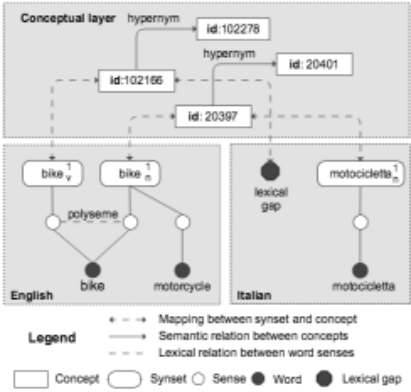
However, differently fromWordNet and its derivatives, 2 the UKC features a conceptual layer fully separated from language. In this layer, concepts are associated unique ids and are connected to language in one of three possible ways: (i) the concept id is mapped (one-to-one) to a synset id, which means that that concept is lexicalized in that language, (ii) the concept id is declared to be a lexical gap for that language, which means that that concept is not lexicalized in that language, and (iii) the concept id is not mapped, which means that we do not know what is the case. A new concept is added only if there is at least a language where it is lexicalized. Furthermore the "usual" lexico-semantic relations (e.g., hypernym, meronym) are embedded in the conceptual layer and connect concept ids, rather than synset ids. The conceptual layer is a kind of semantic layer (in model-theoretic terms, the domain of interpretation of the UKC lexicons) which provides a very powerful means for studying language diversity, while, at the same time, enabling language independent reasoning, as needed, for instance, in cross lingual and language independent applications [Giunchiglia et al., 2012a; Bella et al., 2017].
The overall organization of the UKC is represented in Fig.1. Here, the English word bike has two meanings, as verb and as noun, which are represented by two single word synsets which, through their reference concepts, are connected to the corresponding Italian words. In Italian we have a lexical gap as there is no word for the verb to bike. The two concepts, in turn, are connected in the graph of concepts.
The UKC is in continuous evolution. It is populated via the import of freely available resources, e.g., WordNets or dictionaries, which are preliminarily evaluated to satisfy certain minimal requirements of (very high) quality, or via user input [Giunchiglia et al., 2015]. Some relations in the UKC (e.g., the fact that two senses are homonyms) are generated via reasoning tasks like the one described in this paper. The UKC contains only a very minor number of instances, differently from what is the case in BabelNet and in some applications of the UKC [Giunchiglia et al., 2012b], the main reason being our interest in studying language as such, without "cluttering" it with billions of instances. As a matter of fact, most of the instances present in WordNet have been removed. As of today, the UKC contains 335 languages, 1,333,869 words, 2,066,843 senses, and more than 120,000 concepts where, as it should be expected, no concept is lexicalized in all languages.
2 See, for instance, http://globalwordnet.org.
| #Words | #Languages | Samples |
|---|---|---|
| >90000 | 2 | English, Finnish |
| >75000 | 4 | Mandarin, Japanese, etc. |
| >50000 | 6 | Thai, Polish, etc. |
| >25000 | 17 | Portuguese, Slovak, etc. |
| >10000 | 29 | Islandic, Arabic, et.c |
| >5000 | 39 | Swedish, Korean, etc. |
| >1000 | 66 | Hindi, Vietnam, etc. |
| >500 | 85 | Kazakh, Mongolian, etc. |
| >0 | 335 | Ewe, Abkhaz, etc. |
Table 1 reports the distribution of words over languages. Notice that 90% of the words belong to 50 languages, and that 60% of the languages belong to three phyla (i.e., groups of languages related to one another but less closely than in a family), namely: 115 languages (e.g., Italian) to the IndoEuropean phylum, 52 languages (e.g., Mongolian) to the Ural-Altaic phylum and 36 languages (e.g., Malay) to the Austronesian phylum.
3 Quantifying Language Diversity
The problem of quantifying the diversity of languages is not new, see, e.g., [Bell, 1978; Youn et al., 2016]. Our ideas build upon the work described in [Rijkhoff et al., 1993]. The main goal of this work was to construct balanced datasets with the goal of avoiding linguistic bias. Still sharing the same intuitions, we work in the other direction. Namely, we have the data sets and we measure their diversity in order to exploit it in the solution of well-known linguistic problems.
Diversity has many causes. To name some: genetic ancestry (languages with common origins), geography (due to the influence of physical closeness), culture (effects of cultural dominance). In this paper we present a first attempt at quantifying a global combined diversity measure in terms of genetic diversity and geographic diversity. Given a language set L, we define its combined diversity measure as follows:
In the equation above β ∈ [0, 1] normalizes the effects of genetic diversity over those of geographic diversity. We compute the Relative (Combined) Diversity of two languages by taking |L| = 2 and we (generically) say that two or more languages are similar when they are not diverse and we extend this terminology to all forms of diversity. Let us define the notions of genetic and geographic diversity.
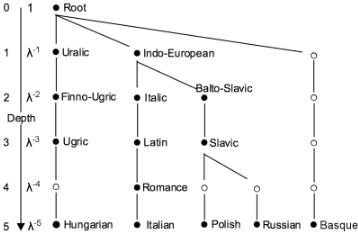
Languages are organized in a Language Family Tree which represents how, in time, languages have descended from other languages, starting from the ancestral languages [Bell, 1978]. A fragment of this tree is shown in Fig.2. This figure must be read as follows. The root is a placeholder for collecting all languages. Labeled intermediate nodes are sets of languages (phyla or families) where the label is the name of the set. Unlabeled intermediate nodes correspond to missing names of language sets and serve the purpose of keeping the tree balanced (crucial for the computation of diversity, see below). Leaves denote languages. In general, we write T (L) to mean the family tree T for the set of languages L (when clear we drop the argument from T ).
The idea behind the computation of genetic diversity is that languages that split closer to the root (that is, further back in time) will have more fundamental changes than those involved in the more recent splits. We capture this intuition by pondering each node n in the Language Family Tree by a real number that decreases with the distance from the root. Thus languages which split very early will generate multiple long branches, thus increasing the overall diversity value. While [Rijkhoff et al., 1993] used linearly decreasing weights, we have chosen the inverse exponential of λ-depth(n) where the depth of the Root is 0 and thus its weight is 1 and where, below it, each phylum is weighted 1/λ, then 1/λ2 , and so on. Furthermore we normalize GenDiv to be in the range [0,1]. More specifically, let T (E) be the family tree of a reference set of languages E, which in our case we take to be the languages in the UKC. Let L ⊆ E be a set of languages for which we want to compute the diversity level and T (L) the corresponding minimal subtree of E. Then, the genetic diversity of L is taken to be 0 if |L| < 2, and, otherwise, defined as:
where AbsGenDiv is what we call the Absolute Genetic Diversity and AbsGenDiv(E) is the Reference Genetic Diversity. To provide some examples, assume we take λ = 2. Then AbsGenDiv(E) = 88.127 and GenDiv(E) = 1, while, with L1 ={Hungarian, Italian, Polish, Russian, Basque} (the languages in Fig. 2) we have AbsGenDiv(L1) = 3.469 and GenDiv(L1) = 0.039. Similarly, if we consider a less diverse subset including only Indo-European languages, e.g., L2 ={Italian, Polish, Russian} we have AbsGenDiv(L2) = 1.531 and GenDiv(L2) = 0.017. In this latter case, adding other Romance languages, e.g., Spanish, Catalan, and Portuguese, to L2 would increase GenDiv only to 0.022, The definition of geographic diversity captures the intuition that languages with speakers living closely to one another tend to share more features and, in particular, a larger portion of their lexicon. This can be explained both diachronically (by the co-evolution of languages) and synchronically (these people will deal with the same types of objects and phenomena). As a first approximation, given that the UKC contains languages from everywhere in the world, we capture this intuition by defining our geographic diversity measure based on the number of different continents on which the languages in the reference data set are spoken. Then, the geographic diversity of L is taken to be 0 if |L| < 2, and, otherwise, defined as:
where continentOf(l) is the continent where l is spoken.
It is important to notice that the computation of geographic diversity through distance metrics alone is a gross oversimplification. Topology and the roughness of terrain, for instance, are important factors: mountain-dwelling people from geographically nearby valleys may in reality be completely isolated from each other. Historical periods of proximity are also ignored by synchronic only approaches, e.g., the temporary mixing of tribes having migrated together through the Eurasian Steppe to then settle at great distances from each other. Still, at this stage, the values of diversity we compute are good enough to produce interesting results.
4 Quantifying Resource Incompleteness
We define two types of incompleteness, i.e., language incompleteness, concept incompleteness and their corresponding measures of coverage plus the notion of ambiguity coverage.
The notion of language incompleteness is a direct extension of the notion of incompleteness of logical languages and theories. Given a reference domain of interpretation, in our case the set of concepts, language incompleteness measures how much of it cannot be named by the elements of the language. We have the following:
where Concepts(l) is the set of concepts denoted by the words in l and Concepts(UKC) is the set of concepts in the UKC (i.e., the concepts denoted by the languages in the UKC). |Concepts(UKC) is decreased by |Gaps(l)|, namely the number of lexical gaps in l to take into account the fact different languages "describe" different worlds. We call AbsLanCov the Absolute Language Coverage. Table 2 (left) organizes the languages of the UKC into four groups, (a), (b), (c), (d), with the first two being highly developed and the latter two being highly under-developed.
The notion of concept incompleteness can be thought of as the dual of language incompleteness. If the latter measures how much of the UKC a language does not cover, the former measures how much a single concept is covered across a selected set of languages. Let, for any concept c, the Languages of c be the set of languages where c is lexicalized, defined as:
where σ(c, l) returns either 1 or 0, depending on whether c is lexicalized in l. Then we define concept coverage and of concept incompleteness as follows:
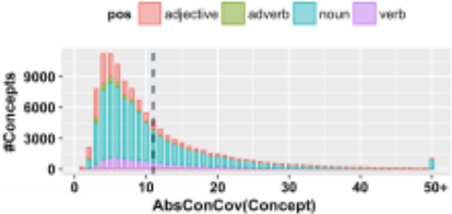
In words: the absolute coverage of a concept is the cardinality of the set of languages where it occurs, its coverage is the absolute coverage normalized over the number of languages of the UKC (defined as Languages(UKC) with a slight abuse of notation), its incompleteness is the complement to 1 of its coverage. Figure 3 shows the distribution of concepts for each value of AbsContCov(Concept) with Concept standing for the sets of the concepts corresponding to the four parts of speech (i.e., adjective, adverb, noun, and verb). As it can be seen from the mean line, on average, concepts are lexicalised across about 10.99 languages.
As it is well known, the key difference between logical languages and natural languages is that the latter, differently from the former, allow words to denote more than one concept. The occurrence of multiple concepts denoted by the same word gives rise to the phenomenon of lexical ambiguity, e.g., polisemy or homonymy. Let the 4-tuple a =<l,w, c1, c2> be an ambiguity instance for l, where c1 and c2 are two concepts expressed by the same word w in the language l. We define the notion of ambiguity coverage as:
The ambiguity coverage of an ambiguity instance measures the level of lexicalization of its concepts in the UKC. The higher this value is the more evidence we have, across languages, towards establishing the type of ambiguity. AmbCov(a) gives us the coverage of a single instance. However, in order to have an overall coverage measure we need to compute, for a given set of languages L, the overall set of ambiguity instances AmbIns(L) and the average ambiguity coverage AvgAmbCov(L), namely the average coverage of instances over the languages in L. We have the following:
| Groups | Language Incompleteness | #Words | #Languages | Sample Languages | #AmbIns | AvgAmbCov |
|---|---|---|---|---|---|---|
| a | LanInc(l) ∈ [0.00; 0.52[ | W ∈ [50, 001;+∞] | 6 | English, Finnish, ... | 714,437 | 10.2 |
| b | LanInc(l) ∈ [0.52; 0.82[ | W ∈ [20, 001; 50, 000] | 15 | Dutch, Spanish, ... | 1,969,436 | 12.8 |
| c | LanInc(l) ∈ [0.83; 0.99[ | W ∈ [501; 20, 000] | 64 | Danish, Albanian, ... | 117,213 | 18.4 |
| d | LanInc(l) ∈ [0.99; 1.00] | W ∈ [1; 500] | 250 | Ewe, Abakhaz, ... | 1,725 | 35.5 |
| UKC | LanInc(l) ∈ [0.00; 1.00] | W ∈ [1;+∞] | 335 | - | 2,802,811 | 12.4 |
In other words, we compute AmbIns(L) by collecting all instances across all languages in L and AvgAmbCov(L) by summing the average coverage of all instances and then by dividing it by the number of these same instances.
Table 2 (right) reports the number of ambiguity instances and their average number for the four language groups plus the UKC. Notice how the average absolute ambiguity coverage is much higher for the under-developed language groups (c), (d). In other words language coverage increases when the average ambiguity coverage decreases, and vice versa: the more developed a resource is the less ambiguity instances we have. This fact, counter-intuitive at first sight, is most probably a consequence of the fact that, in practice, the first words added to a language are the ones which are most commonly used and therefore, the most ambiguous.
5 Polysemy vs. Homonymy
The issue of Lexical Semantic Relatedness has been extensively studied, see, e.g., [Budanitsky and Hirst, 2006]. However, all the work so far has mainly, if not exclusively, concentrated on its study within a single language while we focus on how semantic relatedness propagates across languages. To get an insight into the problem, consider the three examples in Tables 3, 4, 5. These tables provide examples of the types of semantic relatedness we consider. Notice that we distinguish between two types of morphological relatedness: compounding, 3 , namely the combination of free morphemes (as in key+board→keyboard), and derivation namely the combination of a word with one or more derivational affixes (bound morphemes) (as in play+-er→player).
3 We use the term compounding to cover also idioms and collocations where component words are separated by spaces: hot dog, tax cut. This is justified by the fact that the presence or absence of spaces is more a matter of language-specific orthographical convention than a semantic differentiator (e.g., English prefers multiword expressons, German tends to use compounding, whereas some languages such as Chinese do not use spaces to separate words at all).
| # | Language | Concept 1 | Concept 2 | Types |
|---|---|---|---|---|
| 1 | English | bar | bar | polyseme |
| 2 | Italian | barra | bar | derivational |
| 3 | Mongolian | different | ||
| 4 | Chinese | 酒 吧 | 酒 馆 | derivational |
| . . . | . . . | . . . | . . . | . . . |
| 23 | Finnish | baaritiski | baari | compound |
| Types | polyseme | compound | derivational | different |
| Languages | 11 | 1 | 5 | 6 |
Concept 1: a counter where you can obtain food or drink.
Concept 2: an establishment where alcoholic drinks are served over a counter.
| # | Language | Concept 1 | Concept 2 | Types |
| 1 | English | melody, air | air | homonym |
| 2 | Italian | melodia, aria | aria | homonym |
| 3 | Mongolian | different | ||
| 4 | Chinese | 旋律 | 空气 | different |
| . . . | . . . | . . . | . . . | . . . |
| 38 | Turkish | melodi | hava | different |
| Types | homonym | compound | derivational | different |
| Languages | 6 | 0 | 0 | 32 |
Concept 1: a succession of notes forming a distinctive sequence.
Concept 2: a mixture of gases (especially oxygen) required for breathing.
The key observation is that diverse languages represent the same semantic relatedness in diverse ways. Thus, for instance, in Table 3, a polyseme in English corresponds to an occurrence of derivational morphology in Italian and Chinese, to an occurrence of compound morphology in Finnish and to two distinct words in Mongolian.
Our goal is to establish whether any two concepts denoted by a single word are polysemes of homonyms. The algorithm we propose is based on the following intuitions:
- if two concepts are semantically related in diverse languages, then they are polysemes. In this case the diversity of the two languages is evidence of the fact that semantic relatedness derives from a property of the world, which is what all languages denote.
- if two concepts are not semantically related in diverse languages, then they are homonyms. The key idea is that the occurrence of a homonym in a single language, or in similar languages is a coincidence, a consequence of some local, e.g., contextual or cultural, phenomena.
- Similar languages provide little support for the discovery of polysemes and homonyms. At the same time, the existence of polysemes and homonyms can be propagated across similar languages.
But, how do we automatically recognize that two concepts are semantically related? The idea is simple: if we have a big enough number of diverse languages where the two words denoting the two concepts are syntactically similar, then the two concepts are semantically related. A consistent use of the
| # | Language | Concept 1 | Concept 2 | Types |
|---|---|---|---|---|
| 1 | English | tennis | tennis player | compound |
| 2 | Italian | tennist | tennista | derivational |
| 3 | Mongolian | derivational | ||
| 4 | Chinese | 网球 | 网球选 手 | compound |
| . . . | . . . | . . . | . . . | . . . |
| 25 | Korean | _�m��… | _�m��…� �ˆ" | compound |
| Types | polysemy | compound | derivational | different |
| Languages | 0 | 11 | 14 | 0 |
Concept 1: a game played with rackets by two or four players who hit a ball back and forth over a net that divides the court.
Concept 2: an athlete who plays tennis.
similar words is evidence of semantic relatedness, as it also the case in the examples in Tables 3, 5. The resulting algorithm (see algorithm 1) takes in input an ambiguity instance x and a multilingual resource and it returns one of three classifications for x: polyseme, homonym or unclassified. This algorithm is structured as follows:
Step 1. (Lines 1-2). It initializes the set LP of the languages supporting the occurrence of a polyseme (Line 1) and it collects in L all the languages where c1 and c2 are lexicalized (Line 2);
Step 2. (Lines 3-7). It tries to recognize x as a candidate polyseme. This attempt succeeds if one of two conditions hold: (i) the two words are the same, i.e., we have discovered another case of polisemy in a new language or (ii) the two words are morphologically related, as computed by the function morphSim. If it succeeds it adds l to LP .
Our current implementation of morphSim, is a (quite primitive) string similarity metric. For w1 and w2 to be related, morphSim(w1,w2) must return a value higher than a threshold TM. The function len() returns the length of its input while the function LCA() returns the longest common affix (prefix or suffix) of the two input words: for example, 'compet' is the LCA for the words 'compete' and 'competition'. Step 3. (Line 8) It creates the set LH of the languages supporting the occurrence of a homonym. Notice how LH con-
tains the languages where w1 and w2 are different words.
Step 4. (Lines 9-14) x is classified. Notice that, for x, to be classified as a polyseme, the combined diversity of LP must be higher than TD (where "D" stands for Diversity) while, to be classified as a homynm, the combined diversity of LH must be higher than TD and lower than TS (where "S" stands for Similarity). We call TD and TS the Diversity Threshold and the Similarity Threshold, respectively. The intuition is that an ambiguity instance is a polyseme if it occurs in a "diverse enough" language set while it is a homonym if it occurs in a language set where the languages supporting homonymy are "diverse enough" and the languages supporting polisemy are "similar enough". One such example are the two homonyms, one in English and one in Italian, in Table 4.
6 Results
We organize this section in three parts. First we describe how we have learned the hyperparameters. Then we describe the
Input : x =<l, w, c1, c2>, an ambiguity instance Input : R, a multilingual lexical resource Output : label, an ambiguity class for the instance a. 1 LP ← ∅; 2 L← LanguagesR(c1) ∩ LanguagesR(c2); 3 for each language l ∈ L do 4 for each word w1 ∈ WordsR(c1, l) do 5 for each word w2 ∈ WordsR(c2, l) do 6 if w1 = w2 or morphSim(w1, w2) then 7 LP ← LP ∪ {l} ; 8 LH ←L-LP ; 9 if ComDiv(LP ) >TD then 10 label ← 'polyseme' ; 11 else if ComDiv(LH) >TD and ComDiv(LP ) <TS then 12 label ← 'homonym' ; 13 else 14 label ← 'unclassified' ; 15 return label;results of the experiment. Finally we analyze the impact of incompleteness on the experiment itself.
6.1 AlgorithmConfiguration
The hyperparameters to be identified are: the weight β of geographic diversity with respect to genetic diversity, the parameter λ for the computation of genetic diversity, the diversity threshold TD and the similarity threshold TS.
We have computed these values in two steps. First, we have selected a grid of value configurations. The grid has been built by taking, for each parameter, an increment of 0.1 within the following ranges: λ = [1.2; 4.0] (higher values favour more phyla in the language set), TD = [1.0, 10.0] (the higher the value the more diversity is required for polysemy and homonymy detection), TS = [0.3, 1.7] (the lower the value the more similarity is allowed for homonymy), β = [0.0; 1.5] (the lower the less relative significance of geographic diversity), TM = [0.5, 0.8]. The number of configurations which have been analyzed is: 28 (variations on λ) × 90 (variations on TD) × 15 (variations on TS) × 16 (variations on β) × 4 (variations on TM) = 2,419,200 configurations.
Then we have run algorithm 1 with three different methods for computing genetic diversity namely, AbsGenDiv (and not GenDiv: while being conceptually the same, it produced values for β less close to 0), the measure defined in [Rijkhoff et al., 1993] and Baseline, a simple algorithm where an ambiguity instance is classified as a polyseme if L+ contains at least 3 phyla and as a homonym if L+ contains only 1 phylum. In all three cases we have learned the parameters (λ, β, TD, TS, TM) using a training set of 173 polysemes and 146 homonyms from three phyla. Since our ultimate goal is to generate high-quality knowledge, we have favoured precision over recall, setting our minimum precision threshold to 95% and maximising recall with respect to this constraint. The best settings as well as the corresponding precision-recall figures, as computed on the training set, are reported in Table 7. As it can be seen, AbsGenDiv is uniformly better than Rijkhoff's and only loses to Baseline on the recall of homonym classifi-
| Tasks | Resource | Classification Results | ||||
|---|---|---|---|---|---|---|
| Groups | #AmbIns | Groups | AvgAmbCov | Polyseme% | Homonym% | Unclassified% |
| a | 714,437 | a | 4.19 | 13.0 | 43.9 | 43.1 |
| a+b | 2,683,873 | a+b | 10.89 | 30.8 | 21.1 | 48.1 |
| a+b+c | 2,801,086 | a+b+c | 12.40 | 32.4 | 21.2 | 46.4 |
| a+b+c+d* | 2,802,811 | a+b+c+d | 12.43 | 32.4 | 21.2 | 46.4 |
| a | 714,437 | a+b+c+d | 10.28 | 31.6 | 36.1 | 32.1 |
| b | 1,969,436 | a+b+c+d | 12.83 | 31.9 | 14.9 | 53.1 |
| c | 117,213 | a+b+c+d | 18.47 | 46.3 | 29.1 | 24.4 |
| d | 1,725 | a+b+c+d | 35.51 | 71.5 | 16.8 | 11.5 |
| English (a) | 197,502 | a+b+c+d | 9.67 | 32.2 | 22.9 | 44.7 |
| Slovene (b) | 156,317 | a+b+c+d | 12.18 | 35.5 | 27.0 | 37.4 |
| Hungarian (c) | 1,907 | a+b+c+d | 21.67 | 65.7 | 14.9 | 19.2 |
| Haitian (d) | 39 | a+b+c+d | 29.69 | 87.1 | 5.1 | 7.6 |
| Methods | Recall | Homonym Precision | F1 | Recall | Polyseme Precision | F1 |
|---|---|---|---|---|---|---|
| Baseline | 59.58 | 58.00 | 58.77 | 17.64 | 100 | 29.98 |
| Rijkhoff | 12.71 | 95.65 | 22.44 | 11.56 | 95.23 | 20.61 |
| AbsGenDiv | 15.6 | 96.42 | 26.86 | 26.01 | 95.74 | 40.9 |
Baseline: no parameters.
Rijkhoff: β = 1.4, TD = 47.2, TS = 13.2, TM = 0.5.
AbsGenDiv: β = 1.0, TD = 2.52, TS = 0.68, λ = 2.7, TM = 0.5.
cation, which is not relevant, given our focus on precision.
6.2 Polysemy vs. Homonymy
The UKC contains 2,802,811 ambiguity instances across its pool of 335 languages, These instances were automatically generated and then given in input to the algorithm which, in turn, generated 908,110 candidate polysemes and 594,115 candidate homonyms across all languages.
A sample of 640 cases, half being candidate homonyms and half being candidate polysemes, were randomly selected, which were equally divided across seven languages belonging to six different phyla (English, Hindi, Hungarian, Korean, Kazakh, Chinese, Arabic). Seven native speakers were selected as evaluators. All the evaluators, though not being linguists by training, had previously had some exposure to WordNet. They were provided with the glosses of the concepts involved, they were asked the follwing question: "Do you think meanings c1 and c2 of word w are related?", and they had to provide a yes/no answer.
Table 8 provides statistics and accuracy values for each of the languages evaluated. The average accuracy for finding polysemes is 98.3%, even higher than with the training set. Our explanation is that the evaluation dataset is more diverse than the training dataset, as it contains languages from six phyla instead of three. The accuracy of homonym detection is much lower (52.2%), but still significantly higher than what one would obtain by random guessing. At the moment it is unclear whether this lower accuracy is because there are many cases of occurrences of what we call isolated polysemes, namely polysemes occurring in a single language (or a set of similar languages) or, more simply, a consequence of the incompleteness of the UKC. It is a fact that accuracy grows substantially if one increases the number of ambiguity instances considered (see next section). This is a topic for future investigation.
| Accuracy% | |||||
|---|---|---|---|---|---|
| Languages | #Polysemes | #Homonyms | Total | Hom.% | Pol.% |
| English | 50 | 50 | 100 | 48 | 99 |
| Kazakh | 34 | 6 | 40 | 66 | 97 |
| Hungarian | 50 | 50 | 100 | 44 | 100 |
| Hindi | 50 | 50 | 100 | 92 | 98 |
| Chinese | 50 | 50 | 100 | 61 | 100 |
| Korean | 50 | 50 | 100 | 46 | 98 |
| Arabic | 50 | 50 | 100 | 26 | 100 |
| Total | 334 | 306 | 640 | 52.2 | 98.3 |
6.3 The Impact of Resource Incompleteness
We have organized this study following the various steps of the algorithm. Table 6 shows how resource incompleteness impacts the computation of ambiguity instances. It does it in three parts (the three main rows): first by incrementally increasing the languages being analyzed (by adding language groups), then by analyzing the 4 language groups one by one, and finally by analyzing some reference languages. The Tasks column reports the languages being analyzed (thus, for instance (a+b) means all the languages in groups (a) and (b). The Resource column reports the resource over which the analysis is performed. Thus, the first group corresponds to the case where all the languages in the resource are considered; the second group corresponds to the case where the languages in a group are studied in the UKC (namely (a+b+c+d)) while the last group corresponds to the study of single languages in the UKC. The third column provides the classification results.
The overall results show various facts: (i) from the first column, the number of ambiguity instances grows with the size of the languages considered (namely with the total number of words in a language set), as it should be expected; (ii) from the second column, the average number of ambiguity instances increases with the decrease of language coverage also for single languages, thus confirming what discussed in Section 4 (and reported in this table in the second row of this column); (iii) the number of unclassified cases is quite high and decreases with the decrease of the overall language coverage (see second row; remember that group (b) contains many more languages that group (a), see Table 2), which seems coherent with the previous observation.
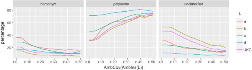
Table 6 links thee average number of ambiguity instances with the classification results. Figure 4 refines this results by showing how, limited to the language groups (a), (b), (c), (d), and the UKC (as reported in the middle of Table 6), the minimal number of ambiguity instances (> 0,> 10,> 20, ...)
| UKC | Classification Results | |||
|---|---|---|---|---|
| AmbCov | #AmbIns | Polyseme% | Homonymy% | Unclassified% |
| >0 | 2,802,811 | 32.4 | 21.2 | 46.4 |
| >10 | 1,805,144 | 41.9 | 14.4 | 43.5 |
| >20 | 325,322 | 55.3 | 11.6 | 32.9 |
| >30 | 44,408 | 64.2 | 11.0 | 24.7 |
| >40 | 9,556 | 71.5 | 10.2 | 18.1 |
| >50 | 3,198 | 73.7 | 10.9 | 15.3 |
which are required for accepting an ambiguity instance as such, impacts the classification results. It shows how, for all the language groups, with the growth of the minimal number of required ambiguity instances, the proportion of homonyms tends to converge to a low percentage (below the 20%), while the proportion of polysemes tends to converge to a very high percentage (above the 70%), and the proportion of unclassified instances decreases substantially (below the 20%). This is coherent with our expectation of a very low percentage of honymyms, most likely below the 10%.
Table 9 provides the numeric quantification of the UKC results graphically represented in Figure 4, together with the extra information of the number of instances computed. It can be noticed how increasing the minimal required number of ambiguity instances consistently increases the percentage of polysemes (up to the 73.7%), decreases the percentage of homonyms (down to the 10.9%) as well as the percentage of unclassified instances (down to around the 15.3%)
Table 10 refines the results in Table 9 by showing how the accuracy with polysemes and homonyms grows with the growth of AmbCov, namely with the growth of the number of languages where the two concepts occurring in an ambiguity instance are lexicalized. It can be seen the accuracy of polysemy is very robust while that of homonymy is highly sensitive to the number of languages, converging to high levels of accuracy.
| Accuracy% | |||||
|---|---|---|---|---|---|
| AmbCov | #Polysemes | #Homonyms | Total | Hom.% | Pol.% |
| >0 | 334 | 306 | 640 | 52.2 | 98.3 |
| >10 | 267 | 297 | 564 | 52.9 | 98.5 |
| >20 | 173 | 143 | 316 | 60.1 | 98.8 |
| >30 | 103 | 33 | 136 | 69.7 | 99.0 |
| >40 | 56 | 10 | 66 | 70.0 | 98.2 |
| >50 | 30 | 7 | 37 | 71.4 | 100.0 |
7 RelatedWork
The universality of linguistic phenomena has been in the focus of historical and comparative linguistics, as well as of the related field of linguistic typology [Croft, 2002]. Universality has been most famously researched on the syntactic level in search of a universal grammar [Evans and Levinson, 2009] but also in the lexicon. Classic quantitative approaches as described in [McMahon and McMahon, 2005], such as lexicostatistics [Swadesh, 1955], mass comparison [Greenberg, 1966], or the recent paper [Youn et al., 2016] on the universality of semantic networks, perform comparisons on relatively small (of up to a couple hundred entries) but very carefully selected word lists expressing the same meaning across a large and unbiased language sample (e.g., the Swadesh list [Swadesh, 1971]). Our research, on the contrary, takes the results of experts on genetic relationships as granted for our diversity measures. Beyond understanding the diversity of the language sets we are working on-and thus evaluating the scope of cross-lingual applicability of our results-we have no a priori reason to exclude certain types of words or phenomena from our experiments and can leverage entire lexicons available to us. The intuition is that the scale of the resource will average out local biases.
The study of polysemy also has a long history, see, e.g., [Apresjan, 1974; Lyons, 1977]. In particular, various computational methods have been proposed for the prediction and generation of polysemy instances from regular (productive) patterns [Buitelaar, 1998; Peters, 2003; Srinivasan and Rabagliati, 2015; Freihat et al., 2016]. Our study goes beyond the limitation of regularity as our goal is not to create rules to be applied over classes of concepts but, rather to find widely recurring polysemy patterns across multiple languages with respect to specific concept pairs.
8 Conclusion
In this paper we have presented a general approach which allows us to use large scale resources, in our case, the UKC, for the solution of relevant language related problems and use the results to improve the UKC itself. The proposed approach has been applied to the discovery of homonyms, as distinct from polysemes, in the UKC. Our current work is concentrated on developing other case studies and on using them to validate and refine the proposed methodology.
@inproceedings{ijcai2017p560,
  title     = {Understanding and Exploiting Language Diversity},
  author    = {Giunchiglia, Fausto and Batsuren, Khuyagbaatar and Bella, Gabor},
  booktitle = {Proceedings of the Twenty-Sixth International Joint Conference on
               Artificial Intelligence, {IJCAI-17}},
  publisher = {International Joint Conferences on Artificial Intelligence Organization},
  editor    = {Carles Sierra},
  pages     = {4009--4017},
  year      = {2017},
  month     = {8},
  note      = {Main track},
  doi       = {10.24963/ijcai.2017/560},
  url       = {https://doi.org/10.24963/ijcai.2017/560},
}
TY - CPAPER TI - Understanding and Exploiting Language Diversity AU - Giunchiglia, Fausto AU - Batsuren, Khuyagbaatar AU - Bella, Gabor T2 - Proceedings of the Twenty-Sixth International Joint Conference on Artificial Intelligence, IJCAI-17 PB - International Joint Conferences on Artificial Intelligence Organization PY - 2017 SP - 4009 EP - 4017 DO - 10.24963/ijcai.2017/560 UR - https://doi.org/10.24963/ijcai.2017/560 ER -Copied
Machine-readable versions of this paper, for tools and AI agents:





