
Locality Constrained Deep Supervised Hashing for Image Retrieval
Proceedings of the Twenty-Sixth International Joint Conference on Artificial Intelligence. Main track. Pages 3567-3573.
https://doi.org/10.24963/ijcai.2017/499
Keywords
- Robotics and Vision: Robotics and Vision
- Machine Learning: Deep Learning
Abstract
Deep Convolutional Neural Network (DCNN) based deep hashing has shown its success for fast and accurate image retrieval, however directly minimizing the quantization error in deep hashing will change the distribution of DCNN features, and consequently change the similarity between the query and the retrieved images in hashing. In this paper, we propose a novel Locality-Constrained Deep Supervised Hashing. By simultaneously learning discriminative DCNN features and preserving the similarity between image pairs, the hash codes of our scheme preserves the distribution of DCNN features thus favors the accurate image retrieval.The contributions of this paper are two-fold: i) Our analysis shows that minimizing quantization error in deep hashing makes the features less discriminative which is not desirable for image retrieval; ii) We propose a Locality-Constrained Deep Supervised Hashing which preserves the similarity between image pairs in hashing.Extensive experiments on the CIFARA-10 and NUS-WIDE datasets show that our method significantly boosts the accuracy of image retrieval, especially on the CIFAR-10 dataset, the improvement is usually more than 6% in terms of the MAP measurement. Further, our method demonstrates 10 times faster than state-of-the-art methods in the training phase.
- [Andoni and Indyk, 2006] Alexandr Andoni and Piotr Indyk. Near- optimal hashing algorithms for approximate nearest neighbor in high dimensions. In FOCS, pages 459-468. IEEE, 2006.
- [Chatfield et al., 2014] K. Chatfield, K. Simonyan, A. Vedaldi, and A. Zisserman. Return of the devil in the details: Delving deep into convolutional nets. In BMVC, 2014.
- [Chopra et al., 2005] Sumit Chopra, Raia Hadsell, and Yann Le- Cun. Learning a similarity metric discriminatively, with appli- cation to face verification. In CVPR, volume 1, pages 539-546. IEEE, 2005.
- [Chua et al., 2009] Tat-Seng Chua, Jinhui Tang, Richang Hong, Haojie Li, Zhiping Luo, and Yantao Zheng. Nus-wide: a real- world web image database from national university of singapore. In ICIVR, page 48. ACM, 2009.
- [Erin Liong et al., 2015] Venice Erin Liong, Jiwen Lu, Gang Wang, Pierre Moulin, and Jie Zhou. Deep hashing for compact binary codes learning. In CVPR, pages 2475-2483, 2015.
- [Gionis et al., 1999] Aristides Gionis, Piotr Indyk, Rajeev Mot- wani, et al. Similarity search in high dimensions via hashing. In VLDB, volume 99, pages 518-529, 1999.
- [Gong and Lazebnik, 2011] Yunchao Gong and Svetlana Lazebnik. Iterative quantization: A procrustean approach to learning binary codes. In CVPR, pages 817-824. IEEE, 2011.
- [Gong et al., 2013] Yunchao Gong, Svetlana Lazebnik, Albert Gordo, and Florent Perronnin. Iterative quantization: A pro- crustean approach to learning binary codes for large-scale image retrieval. PAMI, 35(12):2916-2929, 2013.
- [He et al., 2016] Kaiming He, Xiangyu Zhang, Shaoqing Ren, and Jian Sun. Deep residual learning for image recognition. In CVPR, pages 770-778, 2016.
- [Krizhevsky and Hinton, 2009] Alex Krizhevsky and Geoffrey Hinton. Learning multiple layers of features from tiny images. Master's thesis, Department of Computer Science, University of Toronto, 2009.
- [Krizhevsky et al., 2012] Alex Krizhevsky, Ilya Sutskever, and Ge- offrey E Hinton. Imagenet classification with deep convolutional neural networks. In NIPS, pages 1097-1105, 2012.
- [Lai et al., 2015] Hanjiang Lai, Yan Pan, Ye Liu, and Shuicheng Yan. Simultaneous feature learning and hash coding with deep neural networks. In CVPR, pages 3270-3278, 2015.
- [Li et al., 2016] Wu-Jun Li, Sheng Wang, and Wang-Cheng Kang. Feature learning based deep supervised hashing with pairwise la- bels. AAAI, 2016. IJCAI
- [Lin et al., 2013] Guosheng Lin, Chunhua Shen, David Suter, and Anton van den Hengel. A general two-step approach to learning- based hashing. In ICCV, pages 2552-2559, 2013.
- [Lin et al., 2014] Guosheng Lin, Chunhua Shen, Qinfeng Shi, An- ton van den Hengel, and David Suter. Fast supervised hashing with decision trees for high-dimensional data. In CVPR, pages 1963-1970, 2014.
- [Liu et al., 2012] Wei Liu, Jun Wang, Rongrong Ji, Yu-Gang Jiang, and Shih-Fu Chang. Supervised hashing with kernels. In CVPR, pages 2074-2081. IEEE, 2012.
- [Liu et al., 2016] Haomiao Liu, Ruiping Wang, Shiguang Shan, and Xilin Chen. Deep supervised hashing for fast image retrieval. In CVPR, June 2016.
- [Norouzi and Blei, 2011] Mohammad Norouzi and David M Blei. Minimal loss hashing for compact binary codes. In ICML, pages 353-360, 2011.
- [Raginsky and Lazebnik, 2009] Maxim Raginsky and Svetlana Lazebnik. Locality-sensitive binary codes from shift-invariant kernels. In NIPS, pages 1509-1517, 2009.
- [Russakovsky et al., 2015] Olga Russakovsky, Jia Deng, Hao Su, Jonathan Krause, Sanjeev Satheesh, Sean Ma, Zhiheng Huang, Andrej Karpathy, Aditya Khosla, Michael Bernstein, et al. Ima- genet large scale visual recognition challenge. IJCV, 115(3):211- 252, 2015.
- [Salakhutdinov and Hinton, 2009] Ruslan Salakhutdinov and Geof- frey Hinton. Semantic hashing. IJAR, 50(7):969-978, 2009.
- [Schroff et al., 2015] Florian Schroff, Dmitry Kalenichenko, and James Philbin. Facenet: A unified embedding for face recog- nition and clustering. In CVPR, pages 815-823, 2015.
- [Shen et al., 2015] Fumin Shen, Chunhua Shen, Wei Liu, and Heng Tao Shen. Supervised discrete hashing. In CVPR, pages 37-45, 2015.
- [Simonyan and Zisserman, 2014] Karen Simonyan and Andrew Zisserman. Very deep convolutional networks for large-scale im- age recognition. arXiv preprint arXiv:1409.1556, 2014.
- [Sun et al., 2014] Yi Sun, Xiaogang Wang, and Xiaoou Tang. Deep learning face representation from predicting 10,000 classes. In CVPR, pages 1891-1898, 2014.
- [Torralba et al., 2008] Antonio Torralba, Robert Fergus, and Yair Weiss. Small codes and large image databases for recognition. In CVPR, pages 1-8. IEEE, 2008.
- [Vedaldi and Lenc, 2015] Andrea Vedaldi and Karel Lenc. Matcon- vnet: Convolutional neural networks for matlab. In ACM MM, pages 689-692. ACM, 2015.
- [Wang et al., 2010] Jun Wang, Sanjiv Kumar, and Shih-Fu Chang. Sequential projection learning for hashing with compact codes. In ICML, pages 1127-1134, 2010.
- [Wang et al., 2015] Qifan Wang, Zhiwei Zhang, and Luo Si. Rank- ing preserving hashing for fast similarity search. In AAAI, pages 3911-3917, 2015. IJCAI
- [Weiss et al., 2008] Yair Weiss, Antonio Torralba, and Rob Fergus. Spectral hashing. In NIPS, pages 1753-1760, 2008.
- [Xia et al., 2014] Rongkai Xia, Yan Pan, Hanjiang Lai, Cong Liu, and Shuicheng Yan. Supervised hashing for image retrieval via image representation learning. In AAAI, volume 1, page 2, 2014.
- [Yao et al., 2016] Ting Yao, Fuchen Long, Tao Mei, and Yong Rui. Deep semantic-preserving and ranking-based hashing for image retrieval. AAAI, 2016. IJCAI
- [Zeiler and Fergus, 2014] Matthew D Zeiler and Rob Fergus. Vi- sualizing and understanding convolutional networks. In ECCV, pages 818-833. Springer, 2014.
- [Zhang et al., 2014] Peichao Zhang, Wei Zhang, Wu-Jun Li, and Minyi Guo. Supervised hashing with latent factor models. In SIGIR, pages 173-182. ACM, 2014.
- [Zhu et al., 2016] Han Zhu, Mingsheng Long, Jianmin Wang, and Yue Cao. Deep hashing network for efficient similarity retrieval. In AAAI, 2016.
- [Zhuang et al., 2016] B. Zhuang, G. Lin, C. Shen, and I. Reid. Fast training of triplet-based deep binary embedding networks. In CVPR, 2016.
References were extracted automatically from the PDF and may contain errors.
Full text extracted automatically from the PDF; figures, tables and equations may differ. The PDF is the version of record.
1 Introduction
Due to expensive computational cost and the constraint of bandwidth in network communication, it is very infeasible to directly use raw data for image retrieval among tons of high dimensional data in big data era. Thus Approximate nearest neighbor (ANN) is proposed to solve this problem. As one of the most efficient and effective technique for ANN, hashing draws more and more attention because of its superiority in reducing the cost in terms of time and storage [Torralba et al., 2008] by embedding data onto a hyper-cube (i.e. binary codes) and searching nearest neighbor with hamming distance. For example, only 8MB memory is needed to store 1 million points with 64-bits code, and few milliseconds is needed to search all points. Thus hashing is an extremely useful technique for image retrieval.
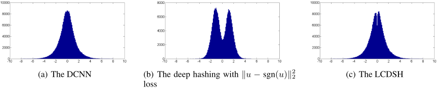
The performance of hashing methods greatly depends on features. For quite a long time, hand-crafted features dominant the computer vision community. By leveraging some elaborately designed features, hashing has shown its good performance in image retrieval [Zhang et al., 2014; Shen et al., 2015; Lin et al., 2013; 2014]. However, such hand-crafted features may not be optimally compatible with hashing methods. Recently deep learning (a.k.a. deep neural network) has demonstrated its great success in many computer vision applications, including image classification [Krizhevsky et al., 2012; Russakovsky et al., 2015; Simonyan and Zisserman, 2014; He et al., 2016], face recognition [Sun et al., 2014; Schroff et al., 2015]. By building a neural network with convolution layer and pooling layer alternatively in a layer-wise manner in Deep Convolutional Neural Networks (DCNN), the learned feature demonstrates its robustness to translation, occlusion, scale, and rotation. In light of the success of DCNN for feature extraction, it also has been introduced to tackle hashing problem, thus deep hashing methods have been proposed [Lai et al., 2015; Li et al., 2016; Zhuang et al., 2016; Liu et al., 2016; Yao et al., 2016; Xia et al., 2014]. Usually, DCNN based hashing can be decomposed into two modules: i) feature learning with DCNN; and ii) feature quantization, i.e., making the DCNN features be close to the binary hashing codes as much as possible. However, As shown in Fig. 2, minimizing the feature quantization error in hashing also changes the feature distribution, thus inevitably reduces the discriminability of features. To make features more discriminative, deeper and deeper networks have been adopted [Liu et al., 2016; Yao et al., 2016; Simonyan and Zisserman, 2014], which in contrast brings additional computational cost, which is against the motivation of hashing.
For image retrieval, it is desirable that the hashing procedure doesn't change the pair-wise similarity between a query and the retrieved images. Therefore it is natural to preserve the pair-wise similarity rather than to minimize the feature quantization error. Motivated by this idea, we propose a Locality-Constrained Deep Supervised Hashing (referred to as LCDSH). Especially, we model the hashing problem as maximizing the posterior probability of the pair-wise label given pair-wise hashing codes, which will be shown to be equivalent to preserve the pair-wise similarity meanwhile make the DCNN features as discriminative as possible. Thus our model is more suitable for image retrieval task than those feature quantization based hashing methods. The main contributions of this paper can be summarized as follows:
- Our study shows that feature quantization based hashing will change the feature distribution, and makes the feature less discriminative.
- We propose a LCDSH. Our strategy not only preserves the discriminability but also preserves the pair-wise similarity, thus our solution is more suitable for image retrieval task. Our solution greatly outperforms all existing methods in terms of both training time and accuracy.
2 RelatedWork
All existing hashing methods can be roughly categorized as data-independent methods [Gionis et al., 1999; Andoni and Indyk, 2006; Raginsky and Lazebnik, 2009] and datadependent methods [Gong and Lazebnik, 2011; Shen et al., 2015]. Compared with the data dependent approaches, dataindependent ones usually need longer codes to achieve similar performance. Therefore, data independent methods don't work well in relative low bits quantization (e.g. 32 and 64 bits)[Andoni and Indyk, 2006]. To avoid the shortcomings of data independent methods, recent research pays more attention to data dependent methods whose hash functions are learned from training data via data-driven methods, which can be further divided into two categories: unsupervised hashing [Gong and Lazebnik, 2011; Gong et al., 2013] and supervised hashing [Lin et al., 2013; 2014; Zhang et al., 2014; Shen et al., 2015; Wang et al., 2015]. Compared with unsupervised methods, the supervised methods are able to utilize class label information to learn more compact hash codes. In the pipelines of most hashing methods for images, each input image is firstly represented by a feature vector of some hand-crafted visual descriptors (e.g., GIST, HOG), followed by a separate projection module (with or without label information) and a quantization module to encode this vector with a binary code.
The label information in supervised hashing can be used in the following three ways: point-wise labels, pair-wise labels, and ranking labels. Representative point-wise label based methods include CCA-ITQ [Gong and Lazebnik, 2011], supervised discrete hashing (SDH) [Shen et al., 2015]. Representative pair-wise label based methods include sequential projection learning for hashing (SPLH) [Wang et al., 2010], minimal loss hashing (MLH) [Norouzi and Blei, 2011], supervised hashing with kernels (KSH) [Liu et al., 2012] twostep hashing (TSH) [Lin et al., 2013], fast supervised hashing (FastH) [Lin et al., 2014], latent factor hashing (LFH) [Zhang et al., 2014]. As for the ranking label based method, ranking preserving hashing (RPH) [Wang et al., 2015] is a very representative one. However, all these methods are based on hand-crafted features [Krizhevsky and Hinton, 2009; Chua et al., 2009].
In light of the success of deep learning in many tasks, including image classification [Krizhevsky et al., 2012; Russakovsky et al., 2015; Simonyan and Zisserman, 2014;
He et al., 2016], face recognition [Sun et al., 2014; Schroff et al., 2015], it also has been introduced to tackle hashing problem. More specifically, deep learning in hashing can be applied in two ways in deep hashing: i) Deep learning is used hashing function learning module, and the features are still based on hand-crafted features. Since the nonlinearity property of deep learning, it has been adopted to approximate the hashing function. The representative work in this category includes [Salakhutdinov and Hinton, 2009; Erin Liong et al., 2015]. However, the hand-crafted features may not be optimally compatible with the hashing module, it is more natural to simultaneously learn the features and hashing functions; ii)Deep learning is used for both feature learning and hashing function. Specifically, [Xia et al., 2014; Lai et al., 2015] have shown that both feature representation and hash coding can be learned simultaneously, and these methods have demonstrated state-of-the-art performance on many benchmarks. However, a disadvantage of these methods is that the quantization error is not statistically minimized hence the feature representation is not optimally compatible with binary hash coding. Recently, some work has been done along this direction, and these methods are usually based on a siamese-liked DCNN architecture to learn features, specifically, both [Li et al., 2016] and [Zhu et al., 2016] employ a pair-wise cross-entropy loss [Zhang et al., 2014] while [Liu et al., 2016] employs a contrastive loss [Chopra et al., 2005] directly. In [Li et al., 2016], authors propose to impose a Gaussian prior on quantization error which is easy to optimize. Both [Zhu et al., 2016] and [Liu et al., 2016] propose a Laplacian prior for quantization. Because Laplacian prior is non-differentiable, [Zhu et al., 2016] adopts a smooth surrogate of the absolute function while [Liu et al., 2016] uses sub-gradients method to optimize the objective function.
3 Approach
3.1 Notation
Suppose there are n points: X = {xi}ni=1 and xi corresponds to the feature of the i-th image, which can either be some hand-crafted features or raw pixel values of the image. We use S = {sij}ni,j=1 (i ̸= j,sij ∈ {-1, 1}) to indicate whether xi and xj belong to the same class: sij = 1 if xi and xj are from the same class, and sij = -1 vice versus.
Deep supervised hashing aims at learning a binary code bi ∈ {-1, 1}ℓ for each point xi, where ℓ is code length. We use B = {bi}ni=1 to denote the hash codes corresponding to points in X. For hashing task, it is desirable that similar images should have similar binary codes. Further, if sij = 1 which means xi and xj are from the same class, it is desirable that the hamming distance between hashing codes bi and bj is low. Otherwise, if sij = -1, the hamming distance between binary codes bi and bj should be high. In general, we can write the hash code as bi = h(xi) = [h1(xi), h2(xi), . . . , hℓ(xi)]T , where h(xi) is a hash function to be learnt.
3.2 ARevisit of Feature Quantization Loss in Deep Hashing
As many traditional hashing methods [Gong and Lazebnik, 2011; Gong et al., 2013], many deep hashing methods also use binarization (feature quantization) to map the continuous features u to hash code b, i.e., b = sgn(u). To reduce the information loss in this binarization operation, most methods minimize the feature quantization error. As far as we know, there are two kinds of quantization minimization strategy in deep hashing: i) ‖sgn(u) - u‖22 [Li et al., 2016]; and ii) ‖‖u‖ - 1‖1 [Zhuang et al., 2016; Zhu et al., 2016]. The difference between them lies on the assumption on the prior distribution of u, i.e., modeling the distribution of each dimensionality of u with a Gaussian Mixture Model or a Laplacian Mixture model. However, such feature quantization loss changes the distribution of u (As shown in Fig. 2), thus may affect the discriminability of the u. For image retrieval, it is desirable that the retrieval results based on b and u should be the same. In other words, the distribution of b and u should be similar in hashing. However, feature quantization loss doesn't agree with such objective very well.
3.3 Network Architecture of LCDSH
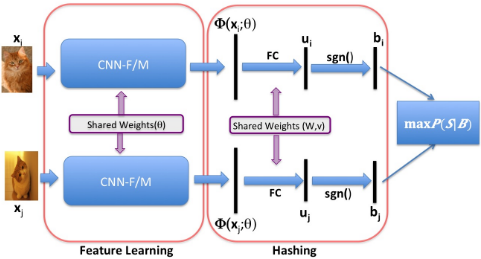
To preserve the pair-wise similarity (locality information) and the discriminability of features in hashing, we propose a Locality-Constrained Deep Supervised Hashing (LCDSH). The network architecture of our LCSH is shown in Fig.1. Specifically, we use a Siamese-liked DCNN, i.e., the two DCNN's are identical. We denote φ(xi; θ) as the output associated with input xi with some DCNN architecture where θ corresponds to the parameters in the feature learning part (parameters in CNN-F/M), φ(xi; θ) ∈ Rd . Here φ(x; θ) works as a feature extractor and any deep learning architecture can be adapted. In this paper we use CNN-F and CNN-M architecture [Chatfield et al., 2014], which would be detailed in implementation section. Then we add one more fully-connected layer to get the feature u, i.e.,
where W ∈ Rd×ℓ denotes a weight matrix, v ∈ Rℓ is a bias vector. To get the hash codes, we use bi = sgn(ui). So the above equation bridges the feature learning part and the hashing part. In training phase, all images are fed into our network in a pair-wise manner with a pair-wise label (sij) indicating whether the image pairs are with the same labels. Our goal is to learn a network that maximizes the posterior probability of P(S|B). Once the network is trained, in the testing phase, we can just feed an image into the network and get its hash codes with a forward pass.
3.4 Loss Function of LCDSH
Our LCDSH both preserves feature discriminative and the locality between image pairs. Specifically, the objective of LCDSH aims at maximizing the following posterior probability:
where maximizing P (S|U) makes the features as discriminative as possible and maximizing P(U|B) preserves the similarity between the features in hashing. Next we will detail these two terms, respectively.
Maximizing P(S|U). Given the features before the binarization in hashing: U = {ui}ni=1 , it is desirable that these features should be as discriminative as possible. Based on the pair-wise label S = {sij}, we define the probability p(sij |ui, uj) = σ(sijΘij), where Θij = 1 2 uTi uj and σ(x) = 1 1+e-x . To make DCNN features discriminative, we can maximize the following objective function:
By taking the negative log-likelihood of the above equation, we arrive at the following equation
We can see that the larger the inner product between ui and uj is, the larger P(1|ui, uj) will be, implying that pair ui and uj should be classified as a similar pair; otherwise, larger P(-1|ui, uj) will imply that ui and uj should be classified as a dissimilar pair.
Maximizing P(U|B). Other than learning discriminative features, LCDSH also aims at preserving pair-wise similarity between images. Thus we model P(U|B) based on the pairwise similarity between images as follows:
where ˜Θij = 1 2 bTi bj,Θij = 12 uTi uj. It is desirable that σ(Θij) is close to σ(˜Θij), then we further let P(σ(Θij)|σ(˜Θij)) be proportional to a Gaussian distribution with variance α, i.e.:
By substituting equation (6) into equation (5) and taking the negative log-likelihood of the equation, the maximizing of P(U|B) is equivalent to the following equation:
Maximize P(S|B). By substituting equation (3) and equation (5) into equation (2), we arrive at the following equation:
By taking the negative log-likelihood of P(S|B), the maximization of P(S|B) is equivalent to the following objective function:
where λ is a trade-off parameter which balances the discriminability and the locality constraint. Our LCDSH simultaneously learns discriminative features and preserves the similarity of image pairs, therefore it is more suitable for retrieval task.
The objective of LCDSH can be optimized efficiently through the standard back-propagation (BP) algorithm. Especially, the gradient of L with respect to ui can be calculated as follows:
where the two terms in equation (11) can be further calculated as follows:
Remarks on Locality-Constraint (P(U|B)). The locality constraint term has several characteristics. First, it plays similar role as quantization in deep hashing. It can be easily shown that that as the loss of L2 decreases, quantization loss also decreases. For example, let ui = [4,-1, 1, 0]T , uj = [-4,-1, 1, 0]T , and then Θij = σ( 12 〈ui, uj〉) ≈ 0 and
˜Θij = 0.6225. It is easy to be observed that 〈ui, uj〉 is good enough to distinguish ui, uj if they are not with the same labels but 〈sgn(ui), sgn(uj)〉 is not a desired distance to discriminate these two embedded vectors.
Second, it is a more general formulation because we do not encourage any prior on the distribution u compared with [Zhuang et al., 2016; Li et al., 2016]. As shown in Fig.2, the Fig.2(a) is the original features distribution of CNN. Basically, it follows a Gaussian distribution. If the feature quantization loss ‖sgn(u)-u‖22 is adopted in deep hashing, then the distribution of u becomes Fig.2(b): two Gaussian distribution centered at 1 and -1, which may affect the discriminability of features. We show the feature distribution of our LCDSH in Fig.2(c), we can see that the distribution of network output is very similar to that of network without quantization loss. But the zero point still can separate the codes as that quantization loss.
Third, because of the sigmoid function, our locality constraint is less sensitive to the large values in features compared with other quantization loss functions. Thus our solution preserves the feature distribution better, and makes the feature more discriminative. For example, if ui = [16,-1, 1, 1,-1,-1, 1,-1]T and uj = [8,-1, 1, 1,-1,-1, 1,-1]T , then Θij = σ( 12 〈ui, uj〉) ≈ 1 and ˜Θij = σ( 12 〈sgn(ui), sgn(uj)〉) = 0.997 This examples shows that such a binary code is good enough to discriminate two points although they have pretty big quantization errors, which demonstrates the robustness of our method.
3.5 Implementation Details
A classical scheme in deep hashing is to fine-tune an image classification model pre-trained on ImageNet by adding a new full-connected layer before the softmax layer. Our model also adopts the same strategy. More specifically, our model has eight layers and the first seven layers are the same as those in VGG-F and VGG-M [Chatfield et al., 2014], which are termed as CNN-F and CNN-M, respectively, and the eighth layer is a fully-connected layer which is used to generate hash codes. The dimensionality of fully connected layer in CNN-F/M (d) is 4096. It is worth noting that any DCNN architecture can be adopted in our framework, but the model of GPU used in our experiments is GTX980-Ti which only has 6GB memory. Therefore we have to choose models like CNN-F, CNN-M rather than VGG-16[Simonyan and Zisserman, 2014] used in [Liu et al., 2016] or VGG-19 used in [Yao et al., 2016], which would cause out of memory issue. Our method is implemented with MatConvNet [Vedaldi and Lenc, 2015]. Our conjecture is that deeper architectures, including VGG-16 and VGG-19, probably correspond to better performance because the features learnt by these networks are more discriminative.
CNN-F architecture is similar to the one used by Krizhevsky et al. in [Krizhevsky et al., 2012]. It comprises of 8 learnable layers, 5 of which are convolutional layers, and the last 3 are fully-connected layers. CNN-M architecture is similar to the one used in [Zeiler and Fergus, 2014]. It is characterized with a larger stride and smaller receptive field in the first convolutional layer, which was shown to be beneficial to image classification on the ImageNet dataset. It is worth noting that larger stride (2 pixels instead of 1 pixel) helps reduce the computational cost and memory.
4 Experiments
4.1 Datasets
We compare our model with several baselines on two widely used benchmark datasets: CIFAR-10 [Krizhevsky and Hinton, 2009] and NUS-WIDE [Chua et al., 2009]. The CIFAR10 dataset consists of 60,000 32×32 color images which are categorized into 10 classes (6000 images per class). It is a single-label dataset in which each image belongs to one of the 10 classes. The NUS-WIDE dataset has nearly 270,000 images collected from the web. It is a multi-label dataset in which each image is annotated with one or multiple class labels from 81 classes. Following [Li et al., 2016; Liu et al., 2016], we only use the images associated with the 21 most frequent classes in our experiments, and the number of images in each class is at least 5000 for these 21 classes.
4.2 Experimental Setup
We compare our method with several state-of-the-art hashing methods. These methods can be categorized into three classes: i) Unsupervised hashing methods with hand-crafted features, including SH [Weiss et al., 2008] and ITQ [Gong and Lazebnik, 2011; Gong et al., 2013]; ii) Supervised hashing methods with hand-crafted features, including, KSH [Liu et al., 2012], FastH [Lin et al., 2013], LFH [Zhang et al., 2014], and SDH [Shen et al., 2015], sequential projection learning for hashing (SPLH) [Wang et al., 2010]; iii) Deep hashing methods, including CNNH [Xia et al., 2014], Network in Network Hashing (NINH) [Lai et al., 2015], Deep Binary Embedding Network (DBEN)[Zhuang et al., 2016], Deep Supervised Hashing (DSH)[Liu et al., 2016], and Deep pair-wise-Supervised Hashing (DPSH) [Li et al., 2016].
For hashing methods with hand-crafted features, we represent the image in CIFAR-10 [Krizhevsky and Hinton, 2009] with a 512-dimensional GIST feature, and represent the image in NUS-WIDE with a 1134-dimensional low-level feature vector, which is comprised of a 64-D color histogram, a 144-D color correlogram, a 73-D edge direction histogram, a 128-D wavelet texture, a 225-D block-wise color moments and a 500-D bag of words based on SIFT descriptions. All these features are provided within the dataset [Chua et al., 2009]. For deep hashing methods, we directly use the raw image pixels as input. We adopt the CNN-F and CNN-M networks pre-trained on the ImageNet dataset [Russakovsky et al., 2015] to initialize the first seven layers of our networks. The Mean Average Precision (MAP) is used to measure the performance of different methods.
4.3 Convergence Speed and Computational Cost
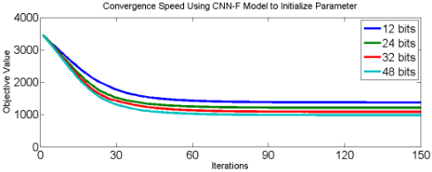
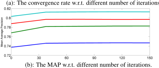
We test the performance of our method with CNN-F model with respect to different number of iterations. We follow existing deep hashing methods [Liu et al., 2016; Zhuang et al., 2016] to fine-tune the model pre-trained on ImageNet, our network converges very fast. Empirically we find that the model converges after about 30 iterations, as shown in Fig. 3-(a). Further, Fig. 3-(b) also shows that the MAP is stable after at about 60 iterations. It is also worth noting that the convergence rate has little relevance to the length of the hash code, and the possible reason is that the change of code length from 12-bits to 48-bits doesn't increase the number of parameters significantly.
| Methods | CIFAR10 | NUSWIDE |
|---|---|---|
| Ours(CNN-F) | 0.5 | 1.5 |
| Ours(CNN-M) | 1.5 | 4.5 |
| DBEN[Zhuang et al., 2016] | 15 | 32 |
| NINH[Lai et al., 2015] | 174 | 365 |
Table 1 shows the training time of different hashing methods with different code lengths on the CIFAR-10 and NUSWIDE datasets, respectively. Here we compare our models with two state-of-the-art methods, including DBEN and NINH, by using the codes provided by authors. Since the codes of other deep hashing methods are not online available, we don't report the training time of those methods. We can see that our model is more than 10× faster than the compared methods. Further, as shown in Table 3 and Table 4, our method achieves much higher MAP than these methods. It is worth noting that our CNN-F model can process more than 1200 images per second for feature extraction by using a GTX980-Ti GPU.
4.4 Sensitivity to Hyper-Parameter λ
In Table 2, we show the performance of our model with respect to different λ on CIFAR-10 dataset. Here we take CNNF as an example. We can see that different λ has little effect on the performance for hash codes with different lengths, which validates the robustness of our model. Further, by comparing Table 2 with Table 3, we can find that our method always outperforms other deep hashing baselines even if we use different λ, which validates the effectiveness of our method.
| λ | 12-bits | 24-bits | 32-bits | 48-bits |
| 0.2 | 0.752 | 0.775 | 0.794 | 0.799 |
| 0.4 | 0.746 | 0.780 | 0.801 | 0.810 |
| 0.6 | 0.742 | 0.794 | 0.797 | 0.808 |
| Method | 12-bits | 24-bits | 32-bits | 48-bits |
|---|---|---|---|---|
| Ours(CNN-F) | 0.752 | 0.794 | 0.801 | 0.810 |
| Ours(CNN-M) | 0.748 | 0.804 | 0.813 | 0.826 |
| DPSH | 0.713 | 0.727 | 0.744 | 0.757 |
| DSH | 0.616 | 0.652 | 0.643 | 0.621 |
| DBEN | 0.650 | 0.760 | 0.765 | 0.770 |
| NINH | 0.552 | 0.566 | 0.558 | 0.581 |
| CNNH | 0.439 | 0.476 | 0.472 | 0.489 |
| FastH | 0.305 | 0.349 | 0.369 | 0.384 |
| SDH | 0.285 | 0.329 | 0.341 | 0.356 |
| KSH | 0.303 | 0.337 | 0.346 | 0.356 |
| LFH | 0.278 | 0.435 | 0.518 | 0.561 |
| SPLH | 0.171 | 0.173 | 0.178 | 0.184 |
| ITQ | 0.162 | 0.169 | 0.172 | 0.175 |
| SH | 0.127 | 0.128 | 0.126 | 0.129 |
4.5 Performance Evaluation
Following [Xia et al., 2014], we randomly select 1000 images (100 images per class) as the query set in CIFAR-10. For the unsupervised methods, we use the rest images as the training set. For the supervised methods, we randomly select 5000 images (500 images per class) from the rest images as the training set. The pair-wise label set S is constructed based on the image class labels and two images will be considered to be similar if they have the same class label.
In NUS-WIDE, we randomly sample 2100 query images from 21 most frequent labels (100 images per class) by following the strategy in [Xia et al., 2014]. For the supervised methods, we randomly select 10500 images (500 images per class) from the rest images as the training set. The pair-wise label set S is constructed based on the image class labels. That is to say, two images will be considered to be similar if they share at least one label. Following the strategy in [Xia et al., 2014], we calculate the MAP based on the top 5000 returned neighbors on the NUS-WIDE dataset.
| Method | 12-bits | 24-bits | 32-bits | 48-bits |
| Ours(CNN-F) | 0.776 | 0.803 | 0.810 | 0.819 |
|---|---|---|---|---|
| DPSH | 0.752 | 0.774 | 0.794 | 0.804 |
| DSH | 0.548 | 0.554 | 0.523 | 0.562 |
| DBEN | 0.650 | 0.745 | 0.760 | 0.775 |
| CNNH | 0.611 | 0.618 | 0.625 | 0.608 |
| NINH | 0.674 | 0.697 | 0.713 | 0.715 |
| FastH | 0.621 | 0.650 | 0.665 | 0.687 |
| SDH | 0.568 | 0.600 | 0.608 | 0.637 |
| KSH | 0.556 | 0.572 | 0.581 | 0.588 |
| LFH | 0.571 | 0.568 | 0.568 | 0.585 |
| SPLH | 0.568 | 0.589 | 0.597 | 0.601 |
| ITQ | 0.452 | 0.468 | 0.472 | 0.477 |
| SH | 0.454 | 0.406 | 0.405 | 0.400 |
The MAP of different methods on CIFAR-10 is reported in Table 3. We can see that our method greatly outperforms other baselines, including unsupervised methods, supervised methods with hand-crafted features, and deep hashing methods with feature learning. It is worth noting that both DPSH and DSH are deep hashing methods with pair-wise labels and feature quantization loss, and our method outperforms these two methods by more than 6%, no matter the length of hash code. In addition, our method even obtains better performance than the method using very deep neural network model [Zhuang et al., 2016]. Meanwhile, since our model benefits from the not-so-deep architecture, the speed of feature extraction of our method is about 10× faster than that of [Zhuang et al., 2016]. The MAP results of NUS-WIDE is reported in Table. 4 1 . We can see that our method always achieves the best performance under all the settings. The good performance of our method on these two datasets validates the effectiveness of our method.
5 Conclusion
Realizing that preserving the locality information is more important in hashing, we propose a Locality-Constrained Deep Supervised Hashing. Specifically, we simultaneously learn discriminative features and preserves the similarity between image pairs in DCNN based hashing. Extensive experimental results validate the effectiveness of our method in terms of the MAP and training time for image retrieval.
1 Here we don't report the performance of CNN-M on NUSWIDE because the model would cause out of memory issue in our experiments.
@inproceedings{ijcai2017p499,
  title     = {Locality Constrained Deep Supervised Hashing for Image Retrieval},
  author    = {Zhu, Hao and Gao, Shenghua},
  booktitle = {Proceedings of the Twenty-Sixth International Joint Conference on
               Artificial Intelligence, {IJCAI-17}},
  publisher = {International Joint Conferences on Artificial Intelligence Organization},
  editor    = {Carles Sierra},
  pages     = {3567--3573},
  year      = {2017},
  month     = {8},
  note      = {Main track},
  doi       = {10.24963/ijcai.2017/499},
  url       = {https://doi.org/10.24963/ijcai.2017/499},
}
TY - CPAPER TI - Locality Constrained Deep Supervised Hashing for Image Retrieval AU - Zhu, Hao AU - Gao, Shenghua T2 - Proceedings of the Twenty-Sixth International Joint Conference on Artificial Intelligence, IJCAI-17 PB - International Joint Conferences on Artificial Intelligence Organization PY - 2017 SP - 3567 EP - 3573 DO - 10.24963/ijcai.2017/499 UR - https://doi.org/10.24963/ijcai.2017/499 ER -Copied
Machine-readable versions of this paper, for tools and AI agents:





