
Multi-Instance Learning with Key Instance Shift
Proceedings of the Twenty-Sixth International Joint Conference on Artificial Intelligence. Main track. Pages 3441-3447.
https://doi.org/10.24963/ijcai.2017/481
Keywords
- Machine Learning: Multi-instance/Multi-label/Multi-view learning
- Machine Learning: New Problems
Abstract
Multi-instance learning (MIL) deals with the tasks where each example is represented by a bag of instances. A bag is positive if it contains at least one positive instance, and negative otherwise. The positive instances are also called key instances. Only bag labels are observed, whereas specific instance labels are not available in MIL. Previous studies typically assume that training and test data follow the same distribution, which may be violated in many real-world tasks. In this paper, we address the problem that the distribution of key instances varies between training and test phase. We refer to this problem as MIL with key instance shift and solve it by proposing an embedding based method MIKI. Specifically, to transform the bags into informative vectors, we propose a weighted multi-class model to select the instances with high positiveness as instance prototypes. Then we learn the importance weights for transformed bag vectors and incorporate original instance weights into them to narrow the gap between training/test distributions. Experimental results validate the effectiveness of our approach when key instance shift occurs.
- [Amores, 2015] Jaume Amores. MILDE: multiple instance learning by discriminative embedding. Knowledge and Information Systems, 42(2):381-407, 2015.
- [Andrews et al., 2002] Stuart Andrews, Ioannis Tsochan- taridis, and Thomas Hofmann. Support vector machines for multiple-instance learning. In Advances in Neural In- formation Processing Systems 15, pages 561-568, 2002.
- [Blei et al., 2003] David M Blei, Andrew Y Ng, and Michael I Jordan. Latent dirichlet allocation. Journal of Machine Learning Research, 3:993-1022, 2003.
- [Chen et al., 2006] Yixin Chen, Jinbo Bi, and James Ze Wang. MILES: Multiple-instance learning via embedded instance selection. IEEE Transactions on Pattern Analysis and Ma- chine Intelligence, 28(12):1931-1947, 2006.
- [Dietterich et al., 1997] Thomas G Dietterich, Richard H Lathrop, and Tomás Lozano-Pérez. Solving the multiple instance problem with axis-parallel rectangles. Artificial Intelligence, 89(1-2):31-71, 1997.
- [Faria et al., 2017] AWC Faria, FGF Coelho, AM Silva, HP Rocha, GM Almeida, AP Lemos, and AP Braga. MILKDE: A new approach for multiple instance learning based on positive instance selection and kernel density esti- mation. Engineering Applications of Artificial Intelligence, 59:196-204, 2017.
- [Ferrer et al., 2010] Geraldo Ferrer, Nicholas Dew, and Uday Apte. When is RFID right for your service ? International Journal of Production Economics, 124(2):414-425, 2010.
- [Gärtner et al., 2002] Thomas Gärtner, Peter A Flach, Adam Kowalczyk, and Alexander J Smola. Multi-instance kernels. In Proceeding of the 19th International Conference on Machine Learning, volume 2, pages 179-186, 2002.
- [Herrera et al., 2016] Francisco Herrera, Sebastián Ventura, Rafael Bello, Chris Cornelis, Amelia Zafra, Dánel Sánchez- Tarragó, and Sarah Vluymans. Multiple Instance Learning: Foundations and Algorithms. Springer, 2016.
- [Huang et al., 2006] Jiayuan Huang, Arthur Gretton, Karsten M Borgwardt, Bernhard Schölkopf, and Alex J Smola. Correcting sample selection bias by unlabeled data. In Advances in Neural Information Processing Systems 19, pages 601-608, 2006.
- [Kanamori et al., 2009] Takafumi Kanamori, Shohei Hido, and Masashi Sugiyama. A least-squares approach to di- rect importance estimation. Journal of Machine Learning Research, 10:1391-1445, 2009.
- [Li et al., 2009] Yu-Feng Li, James T Kwok, Ivor W Tsang, and Zhi-Hua Zhou. A convex method for locating regions of interest with multi-instance learning. In Proceeding ot 20th European Conference on Machine Learning, pages 17-32, 2009.
- [Maron and Lozano-Pérez, 1998] Oded Maron and Tomás Lozano-Pérez. A framework for multiple-instance learning. In Advances in Neural Information Processing Systems 10, pages 570-576, 1998.
- [Senta et al., 2007] Yosuke Senta, Yoshihiko Kimuro, Syuhei Takarabe, and Tsutomu Hasegawa. Machine learning ap- proach to self-localization of mobile robots using RFID tag. In Proceedings of the IEEE/ASME International Con- ference on Advanced Intelligent Mechatronics, pages 1-6, 2007.
- [Shimodaira, 2000] Hidetoshi Shimodaira. Improving pre- dictive inference under covariate shift by weighting the log-likelihood function. Journal of Statistical Planning and Inference, 90(2):227-244, 2000.
- [Sugiyama et al., 2008] Masashi Sugiyama, Shinichi Naka- jima, Hisashi Kashima, Paul V Buenau, and Motoaki Kawanabe. Direct importance estimation with model se- lection and its application to covariate shift adaptation. In Advances in Neural Information Processing Systems 21, pages 1433-1440, 2008.
- [Sugiyama et al., 2012] Masashi Sugiyama, Taiji Suzuki, and Takafumi Kanamori. Density Ratio Estimation in Machine Learning. Cambridge University Press, 2012.
- [Wei et al., 2017] Xiu-Shen Wei, Jianxin Wu, and Zhi-Hua Zhou. Scalable algorithms for multi-instance learning. IEEE Transactions on Neural Networks and Learning Sys- tems, 28(4):975-987, 2017.
- [Yuan et al., 2016] Jiazheng Yuan, Xiankai Huang, Hongzhe Liu, Bing Li, and Weihua Xiong. Submil: Discriminative subspaces for multi-instance learning. Neurocomputing, 173:1768-1774, 2016.
- [Zadrozny, 2004] Bianca Zadrozny. Learning and evaluating classifiers under sample selection bias. In Proceeding of the 21st International Conference on Machine Learning, pages 114-121, 2004.
- [Zhang and Zhou, 2014] Wei-Jia Zhang and Zhi-Hua Zhou. Multi-instance learning with distribution change. In Pro- ceeding of the 28th AAAI Conference on Artificial Intelli- gence, pages 2184-2190, 2014.
- [Zhang et al., 2002] Qi Zhang, Sally A Goldman, Wei Yu, and Jason E Fritts. Content-based image retrieval using multiple-instance learning. In Proceeding of the 19th Inter- national Conference on Machine Learning, pages 682-689, 2002.
- [Zhou et al., 2005] Zhi-Hua Zhou, Kai Jiang, and Ming Li. Multi-instance learning based web mining. Applied Intelli- gence, 22(2):135-147, 2005.
- [Zhou et al., 2009] Zhi-Hua Zhou, Yu-Yin Sun, and Yu-Feng Li. Multi-instance learning by treating instances as non-iid samples. In Proceeding of the 26th International Confer- ence on Machine Learning, pages 1249-1256, 2009.
References were extracted automatically from the PDF and may contain errors.
Full text extracted automatically from the PDF; figures, tables and equations may differ. The PDF is the version of record.
1 Introduction
Multi-instance learning (MIL) [Herrera et al., 2016] deals with the tasks where each example is represented by a bag of instances. A bag is positive if it contains at least one positive instance, and negative otherwise. The instances that trigger the positive labels are also called key instances. Only bag labels are observed, whereas instance labels are unknown in MIL. MIL has been applied in many domains, including image classification [Zhang et al., 2002], text categorization [Andrews et al., 2002], and web mining [Zhou et al., 2005], etc.
Previous studies of MIL typically assume that the training and test data are drawn from the same distribution, which may be violated in many real-world tasks. The distribution discrepancy may arise when training and test data are collected in different time, location or with different labeling cost, etc.
∗This research was supported by the NSFC (61333014) and Huawei Fund (YBN2017030027).
Take text categorization for example, supposing that we want to judge whether a text is about 'sport' and the training/test data are collected in 2012/2016, respectively. Then compared with training data, test data may have less texts about 'Kobe Bryant', but more about 'Stephen Curry'. Here the paragraphs containing 'Kobe Bryant' or 'Stephen Curry' can be regarded as key instances. In this case, the distribution of key instances changes between training and test phase due to different collection time. Also, if the training/test data are collected in America/China respectively, then compared with training data, test data may have less texts about 'baseball', but more about 'table tennis'. Here the paragraphs with 'baseball' or 'table tennis' can be regarded as key instances. The distribution of key instances varies due to different collection locations. In this paper, we formalize this problem as MIL with key instance shift and propose the MIKI (Multi-Instance with Key Instance shift) method to solve it.
MIKI follows the embedding based manner [Chen et al., 2006], which transforms bags into single instance vectors via embedding. Instance prototypes are selected to encode both bag-level information and key instance shift information. First, a weighted multi-class model is trained to select the instances with high positiveness as instance prototypes, and the bags are transformed into informative vector representations with selected instance prototypes. Then, we learn the weights for the transformed bag vectors and incorporate the original instance weights into them to narrow the gap between training/test distributions. Finally, a model is learned by using the new representations and their weights. Experiments on different data sets demonstrate the effectiveness of our approach when key instance shift occurs. Even without key instance shift, MIKI still works comparable with the state-of-the-art methods.
The rest of this paper is organized as follows. Section 2 reviews related work. Section 3 presents the proposed method. Section 4 reports the experimental results. Section 5 applies the proposed method to moving object localization problem and Section 6 concludes.
2 RelatedWork
Multi-instance learning was first proposed in [Dietterich et al., 1997]. Since then, many approaches have been proposed, which mainly fall into two categories: some try to directly solve the MIL problem in either instance level [Maron and Lozano-P´erez, 1998; Li et al., 2009; Faria et al., 2017] or bag level [G¨artner et al., 2002; Zhou et al., 2009], while the others transformMIL into single instance learning via embedding, among which MILES [Chen et al., 2006] is a typical representative, and many methods [Amores, 2015; Yuan et al., 2016; Wei et al., 2017] have been proposed recently following this manner. It is noteworthy that previous MIL methods typically assume that the training and test data follow the same distribution. In contrast, we consider the key instance shift problem, which has not been thoroughly studied to our best knowledge.
In addition, due to the differences in gathering data, distribution change between training and test data may always arise, among which covariate shift [Shimodaira, 2000] has attracted much attention. In covariate shift, the input distribution P(x) is different between training and test phase but the conditional distribution of output P(y|x) remains unchanged. A common approach for covariate shift is importance reweighting, which assigns each training instance x with a weight w(x) = pte(x)/ptr(x) to diminish the discrepancy of training and test marginals by some criteria [Sugiyama et al., 2012]. Note that test data is needed to estimate the difference of distribution. Many methods have been proposed to estimate the weight, such as KMM [Huang et al., 2006], KLIEP [Sugiyama et al., 2008], LSIF and uLSIF [Kanamori et al., 2009], etc. However, all of these studies focus on single-instance learning.
The most related literature of our work is [Zhang and Zhou, 2014], which considers the setting when MIL encounters distribution change and proposes the MICS method. In contrast to considering situations where the bag label is decided by multiple instances and their relations [Zhang and Zhou, 2014], in this paper, we follow the standard MIL setting that bag labels are determined by the key instances, and consider the distribution change problem of key instances.
3 MIL with Key Instance Shift
3.1 Problem Statement and Notations
Let X = Rd denote the instance space and Y = {-1,+1} denote label space. The learner is given a data set with m training bags Btr = {(Xtr 1 , y1), . . . , (Xtr i , yi), . . . , (Xtr m , ym)}, where Xi = {xi1, . . . , xij , . . . , xini } is a bag with xij ∈ X representing an instance. If there exists any positive instance in Xi, then Xi is a positive bag with yi = +1; otherwise Xi is negative with yi = -1. Those positive instances are also called key instances, which trigger the positive labels. Note that only bag labels are available, yet specific instance labels are unknown. The learner is also given a set of n unlabeled test bags Bte = {Xte 1 , . . . ,X te n }. In MIL with key instance shift problem, the distributions of key instances in training and test phase are different. Let P(·) denote the distribution, x∗ refer to the key instances, then we have P(xtr ∗ ) ̸= P(xte ∗ ) in this setting. In this work, we focus on transductive setting: given Btr and Bte, where P(xtr ∗ ) ̸= P(xte ∗ ), our goal is to learn a mapping f : 2X → Y that works fine for test data.
3.2 ProposedMethod
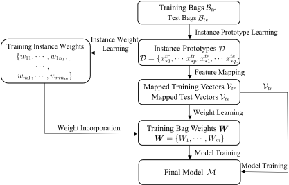
MIKI follows the embedding based manner [Chen et al., 2006], which transforms bags into single instance vectors via embedding. To handle the key instance shift problem, we try to select key instance candidates from both training and test sets as instance prototypes so that both bag-level information and key instance shift information can be encoded. Specifically, assuming that the positive instances belong to different subconcepts, then key instance shift may fall into any of these sub-concepts. Supposing that there are K sub-concepts, together with the negative concept, we build a (K + 1)-class model to distinguish different sub-concepts and the negative concept. If an instance belongs to any sub-concept with a high score, it would be regarded as a key instance candidate with high probability. In this way, different shift information can be captured. Moreover, in order to alleviate the influence of key instance shift, we introduce the instance weights to balance different distributions (i.e., higher/lower weights for underrepresented/overrepresented instances), so that the selected instance prototypes may include more key instances and encode more key instance shift information. Similarly, after getting the transformed bag vectors, we learn the weights for them to narrow the gap of training/test distributions. Note that if an instance is important, the bag containing it should also be valued, so we further incorporate weights of the original instances into the weights of the transformed bag vectors. The final model is learned with the transformed bag vectors and their weights. Figure 1 summarizes our MIKI approach.
Instance Prototype Learning
In instance prototype learning phase, a weighted multi-class model is trained to select key instance candidates as instance prototypes. We use an iterative framework to alternately build the multi-class model and optimize the selected key instance candidates, and then update the instance weights 1 . Algorithm 1 summarizes the instance prototype learning framework.
Specifically, in each iteration, a weighted (K + 1)-class model MD is trained for the K sub-concepts of positive instances and the negative concept. If an instance belongs to any sub-concept with a high score, it would be regarded with high positiveness. To represent the positiveness, we denote the probability of instance xij belonging to class k as Prk ij , and calculate the positiveness score Sij for each instance xij:
1 The importance weighting technique is same to the one introduced in the next section.
Algorithm 1 Instance Prototype Learning for MIKI
Input: Training bags Btr = {(Xtr i , yi)}mi=1, Testing bags Bte = {Xte j }nj=1, Instance selection parameters ntr θ and nte θ .
Output: Instance Prototype Set D.
- 1: Initialize all training instance weights w.
- 2: repeat
- 3: Train multi-class modelMD by Algorithm 2;
- 4: Calculate positiveness score for all instances by Eq. 1;
- 5: Separate instances into Ctr p , Ctr n , Cte p and Cte n by Eq. 4;
- 6: Reestimate the weights wp (wn ) for instances in Ctr p (Ctr n ) to approximate instances in Cte p (Cte n );
- 7: until max iteration is reached.
- 8: Output D = Cp tr ∪ Cp te .
Algorithm 2 shows the details of learning MD. We first run k-means on all instances from positive bags and initialize their labels as the associated cluster numbers, and assign all instances from negative bags with label 0. A multi-class SVM model M is trained with the weighted instances and their assigned labels. Given an instance xij, the model Mwill output the probability Prk ij of xij belonging to class k. Then for each instance xij from positive bags, its label is updated to be
The labels of instances in negative bags stay unchanged. For each positive bag Xi, if all instances are labeled negative, the label of the instance (denote as xip) with the highest positiveness score is adjusted to be
so that each positive bag contains at least one positive instance and the initialized false positives are calibrated through iteration. The step sequence interleaves until no label changes or max iteration is reached, then the model MD is obtained.
With the obtained model MD, the positiveness score of each instance is estimated and key instance candidates are selected. Specifically, let Str θ (Ste θ ) denote the ntr θ -th (nte θ -th) highest score of all training (test) instances, we then separate the instances into key instance candidates and negative instance candidates according to their positiveness scores:
Here, C tr p and C te p are those instances with higher positiveness scores, so they are more likely to be potential key instances and carry the key instance shift information.
After the separation, we reestimate the weights for training instances in key (negative) instance candidates correspondingly, i.e., reestimate the weights for C tr p (C tr n ) by using C te p (C te n ). Thus, all training instance weights are updated. Then the model MD will be trained again with updated weights and the key instance candidates will be updated. This step sequence interleaves until the max iteration is reached, and the
Algorithm 2 Learning algorithm for multi-class model MD
Input: Training bags Btr = {(Xtr i , yi)}mi=1, Training instance weights w, Positive cluster number K.
Output: Multi-class modelMD
- 1: Initialize the labels for all training instances;
- 2: repeat
- 3: Train multi-class model with the weighted training instances;
- 4: Update the labels of all instances from positive bags by Eq. 2;
- 5: For each positive bag, if all instances are labeled negative, select the most positive one and adjust its label by Eq. 3;
- 6: until no label changes or max iteration is reached.
- 7: Output the final model asMD.
selected instance prototypes (i.e., C tr p ∪C te p ) are outputted as instance prototype set D.
With D, we map both training and test bags into new vector representations following the typical procedure [Chen et al., 2006]. Concretely, each bag Xi is mapped into a (ntr θ +nte θ )- dimensional vector vi, and the j-th attribute vij is
where Dj is the j-th term of D. The new representations keep both bag-level information and key instance shift information.
Weight Learning
In this section, we present the details of learning the weights for transformed training vectors. Given transformed training vectors {vtr i }mi=1 with density ptr(v) and transformed test vectors {vte i }ni=1 with density pte(v), we want to estimate the importance w(v) = pte(v)/ptr(v) for all transformed training vectors. Following [Kanamori et al., 2009], we model the weight w(v) by the following linear model:
where α = (α1, . . . , αb)T are parameters to be learned and {ϕl(v)}bl=1 are basis functions satisfying ϕl(v) ≥ 0 for all v and l. Here we choose a fixed number of Gaussian kernels centered at test points as the basis functions. We need to estimate the parameters {αl}bl=1 to make ˆw(v) approximate to w(v). To achieve this, we minimize the following squared error L0(v):
since the last term in Eq. 7 is a constant given the training set, it can be safely ignored. Using pte(v) = w(v)ptr(v), we denote the first two terms by L(v):
Approximating to the expectations in L(v) by empirical averages, we obtain ˆL(v):
where ˆH is the b×b matrix with the (l, l′ )-th element ˆHl,l′ = ∑mi=1 ϕl(vtr i )ϕl′(vtr i )/m and ˆh is the b-dimensional vector with the l-th element ˆhl = ∑nj=1 ϕl(vte j )/n. Based on Eq. 9, we get the following optimization problem:
Eq. 10 is an unconstrained convex quadratic program, so the solution can be analytically computed as α = ( ˆH + λIb)-1ˆh, where Ib is the b-dimensional identity matrix, thus the parameters can be efficiently estimated and the weight of each training sample can be obtained. This importance weighting technique is exactly the one used in Algorithm 1 with v replaced by x.
With the aforementioned method, we can get the weights for all transformed training vectors, and we denote the weights as W 0 . Moreover, we address that if a bag contains an instance that should be valued, the bag should be valued too, thus we further incorporate instance weights into the transformed bag weights. Note that when we learn the instance prototypes, the instances are separated into C tr p (C te p ) and C tr n (C te n ) according to their positiveness. We follow the same procedure to learn the weights for instances in C tr p (C tr n ) to approximate the instances in C te p (C te n ), separately. Thus, all training instance weights are estimated and they are further integrated into the transformed bag weights. Concretely, for training bag Xtr i and its transformed vector vtr i , denote the weight learned from the transformed bag vectors as W 0 i and the weights for instances in this bag as {wij}ni j=1 , the final weight of vtr i is set to be:
At the end of MIKI, we use the transformed training feature vectors and their corresponding weights to learn the classification model, which is employed it to classify the transformed test feature vectors.
Note that the number of selected instance prototypes in MIKI is much smaller than that used in MILES and many other embedding based methods, and thus, MIKI is more efficient in this aspect. The iterative instance prototype learning process of MIKI is similar to miSVM [Andrews et al., 2002], and thus, mechanisms for time cost control and acceleration for miSVM can be applied.
4 Experiments
The experiments are performed on both synthetic data and real world datasets. We compare the proposed method with many state-of-the-art algorithms, including instance-level methods miSVM and MISVM [Andrews et al., 2002], and bag-level methods miGraph [Zhou et al., 2009], MILES [Chen et al., 2006] and MILDE [Amores, 2015]. We also derive three variants for comparison. The first one miSVM+, works by estimating the weights for all instances, and incorporating them directly to miSVM. The second one MILES+, is a variant of MILES and the weights are obtained based on the transformed feature vectors. In addition, since we have used instances from test bags in MIKI, we derive the third variant MILES++, using all instances from both training and test bags for feature mapping with importance weighting technique incorporated. Furthermore, we also compare with MICS [Zhang and Zhou, 2014], which focuses on the setting of MIL with distribution change. RBF kernel is used for all SVM-based methods. For MIKI, we simply set K to 5 for synthetic dataset and 10 for the other datasets without any tuning, and set max iteration to 5 to accelerate the method. Other parameters are selected via 5-fold cross validation.
4.1 Experiments on Synthetic Data
We first perform experiments on synthetic dataset. We generate two sub-concepts of positive instances which are represented by Gaussian distribution P1 = N(µ1, σ2 ) and P2 = N(µ2, σ2 ), and one negative concept represented by P3 = N(µ3, σ2 ). Here we set µ1 = (1, 1), µ2 = (2, 2), µ3 = (3.5, 2.5), σ2 = (0.5, 0.5). Each bag contains 10 instances, and each positive bag contains 1 positive instance, which is from one of the sub-concepts (i.e., P1 or P2). We generate 200 negative and 200 positive bags. Half of the positive bags contain positive instances from one sub-concept, and the other half from another.
We follow the typically deliberately biased sampling procedure [Zadrozny, 2004] to separate the bags into disjoint training and test sets. Specifically, we define a random variable si for each bag, where si = 1 means that the i-th bag is selected into training set, and si = 0 otherwise. For positive bag Xi, denote the key instance as xi∗, then the positive bags are sampled following the rules below:
Here, SC1 and SC2 denote different sub-concepts (i.e.,P1 and P2) and a = 0.8, b = 0.2. In other words, compared with test data, there are more positive bags in training data containing positive instances from sub-concept P1, but less from P2.
We repeat experiments for 30 times by using the sampling procedure to generate training and test sets. As shown in Table 1, our method outperforms all other ones. Though distribution change is considered, miSVM+, MILES+ and MILES++ do not show significant improvement, verifying that simply applying single-instance distribution shift approaches to MIL does not work. MICS does not get favorable result too.
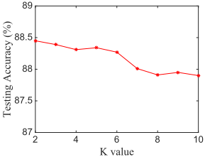
Furthermore, we examine the influence of parameter K. In MIKI, we simply set K to 5, but not the ground-truth number of sub-concepts. The results in Figure 2 show that the behavior tends to get better as the value of K getting closed to the ground-truth. However, our method is not that sensitive to K. Moreover, we observe that almost 88% of the selected instance prototypes of MIKI are positive, verifying the effectiveness of selecting 'positive' instances in MIKI.
| miSVM | MISVM | miGraph | MILES | MILDE | miSVM+ | MILES+ | MILES++ | MICS | MIKI | |
|---|---|---|---|---|---|---|---|---|---|---|
| Accuracy | 77.2±1.7 | 82.6±1.3 | 81.4±1.9 | 83.4±1.9 | 83.7±1.4 | 80.3±1.4 | 83.0±2.0 | 83.0±2.1 | 78.8±4.5 | 88.3±1.1 |
4.2 Experiments on Text Categorization
We then perform experiments on text categorization tasks. We derive 25 data sets from the popularly used 20 Newsgroups corpora. The documents belong to 6 main classes and 20 subclasses. For each dataset, we set one main class (e.g., 'comp') as positive, and the others as negative. For positive class, two sub-classes (e.g., 'comp.sys.ibm.pc' and 'comp.windows.x') are used as different sub-concepts. 200 positive and 200 negative bags are generated. Each positive bag contains averagely 1.5 instances from positive class, and the negative instances are randomly and uniformly drawn from the negative classes. Half of the positive bags contain positive instances from one sub-concept, and the other half from another sub-concept. An instance is a post represented by 100-dimensional LDA feature [Blei et al., 2003].
Similarly, the biased sampling procedure is used to separate bags. Eq. 12 is used to sample the bags, with SC1 and SC2 being different sub-classes, and a = 0.8, b = 0.2. Thus, compared with test data, there are more positive instances in training bags from SC1, but less from SC2.
We repeat experiments for 30 times by using the sampling procedure to generate training and test sets. The results are reported in Table 2, with the win/tie/loss counts in the last row. As we can see, MIKI achieves 22 times the best performance, which is significantly better than other algorithms. MICS does not work well because as we have mentioned in the end of related work, it is designed to handle other types of distribution shift rather than key instance shift. It is interesting to see that miSVM+ and MILES+/MILES++ are not necessarily better than miSVM and MILES, respectively. This suggests that a simple extension by applying single-instance distribution shift approach does not work. One important reason is that in multi-instance learning there is no accurate information of instance label, and thus, instance weighting approach which is effective for single-instance setting may become misleading in multi-instance setting.
| Instance-level method | Bag-level method | Variant of state-of-the-art method and distribution change method | Proposed method | |||||||
|---|---|---|---|---|---|---|---|---|---|---|
| miSVM | MISVM | miGraph | MILES | MILDE | miSVM+ | MILES+ | MILES++ | MICS | MIKI | |
| comp gra ibm | 64.0±5.1 | 59.9±7.6 | 69.9±4.7 | 67.7±3.8 | 68.9±3.7 | 63.7±4.9 | 67.4±4.1 | 67.6±4.1 | 69.7±4.8 | 74.1±5.2 |
| comp gra mac | 62.8±4.6 | 61.1±8.0 | 65.7±3.4 | 69.1±4.5 | 67.7±3.8 | 62.9±4.4 | 68.2±5.0 | 69.6±4.1 | 65.1±3.0 | 71.1±4.9 |
| comp gra os | 79.0±3.0 | 63.5±10.9 | 75.0±3.3 | 78.7±2.9 | 80.1±2.8 | 79.1±3.0 | 78.7±3.0 | 78.6±3.1 | 74.4±3.3 | 82.5±3.3 |
| comp gra win | 76.0±4.7 | 62.2±7.1 | 70.9±3.1 | 75.2±3.0 | 76.7±3.2 | 76.0±4.3 | 75.3±3.3 | 75.8±3.5 | 69.7±5.3 | 79.0±3.5 |
| comp ibm mac | 73.6±5.1 | 62.4±10.7 | 72.2±3.6 | 77.0±3.0 | 78.1±2.8 | 73.9±5.0 | 76.9±2.7 | 77.2±3.2 | 72.2±3.9 | 79.2±2.7 |
| comp ibm win | 69.6±4.5 | 56.0±5.2 | 68.7±4.0 | 69.3±3.3 | 65.9±4.0 | 70.2±4.2 | 66.4±4.5 | 68.4±4.3 | 68.9±4.0 | 77.9±4.7 |
| comp mac win | 67.9±6.7 | 57.9±5.3 | 65.0±3.9 | 63.7±4.4 | 63.1±3.3 | 66.5±7.9 | 63.9±5.1 | 67.4±4.2 | 65.0±3.8 | 76.5±4.8 |
| comp os ibm | 70.1±5.2 | 62.1±9.0 | 73.6±3.7 | 71.6±2.8 | 71.7±4.5 | 69.8±5.3 | 71.6±3.0 | 72.0±3.7 | 74.0±3.6 | 79.3±3.5 |
| comp os mac | 68.3±6.7 | 62.2±9.6 | 70.4±3.4 | 73.0±3.5 | 74.0±3.6 | 67.5±7.1 | 72.9±3.7 | 73.1±3.8 | 69.9±3.8 | 76.9±3.0 |
| comp os win | 77.3±3.7 | 62.8±9.8 | 71.8±3.7 | 75.1±3.1 | 76.5±2.7 | 77.4±3.4 | 75.8±3.2 | 75.1±2.8 | 71.9±3.7 | 79.8±4.0 |
| rec auto baseball | 68.8±9.8 | 58.0±5.4 | 63.0±5.1 | 63.2±6.3 | 58.7±3.8 | 69.1±9.6 | 60.1±5.9 | 69.8±5.4 | 62.2±4.8 | 81.1±4.4 |
| rec auto hockey | 78.4±9.9 | 61.6±7.3 | 64.0±3.2 | 70.3±5.7 | 59.6±3.4 | 78.2±9.7 | 68.7±6.1 | 71.5±7.0 | 63.0±4.2 | 85.6±3.9 |
| rec auto moto | 59.0±5.8 | 57.3±4.0 | 59.8±3.6 | 63.0±2.6 | 64.6±3.7 | 57.6±4.8 | 63.1±2.6 | 63.0±2.5 | 59.7±4.0 | 68.9±4.9 |
| rec baseball hockey | 92.0±2.4 | 74.9±4.9 | 73.8±4.0 | 87.4±2.7 | 89.1±2.2 | 92.2±2.3 | 88.4±2.3 | 88.6±2.9 | 73.6±4.0 | 93.8±2.0 |
| rec moto baseball | 62.5±5.9 | 59.5±5.0 | 59.6±3.2 | 66.2±3.8 | 71.5±6.6 | 62.7±6.1 | 66.0±3.8 | 65.8±4.5 | 59.4±3.7 | 74.6±6.8 |
| rec moto hockey | 71.1±7.5 | 61.6±7.4 | 62.5±3.9 | 67.6±5.2 | 77.7±5.3 | 70.9±7.1 | 69.4±4.2 | 71.9±3.9 | 63.5±3.1 | 83.0±3.3 |
| sci crypt elec | 57.3±3.4 | 54.2±3.7 | 56.2±3.6 | 58.5±2.5 | 60.1±2.2 | 57.4±3.0 | 59.2±2.1 | 59.4±2.5 | 55.4±3.9 | 59.3±3.4 |
| sci crypt med | 58.1±4.0 | 55.7±3.7 | 58.4±4.4 | 59.8±3.8 | 58.1±2.3 | 57.9±3.4 | 60.1±4.3 | 63.0±4.2 | 58.0±4.2 | 66.3±6.6 |
| sci crypt space | 56.1±2.0 | 55.3±4.0 | 55.1±4.8 | 58.6±2.1 | 58.7±2.3 | 56.9±1.4 | 59.1±2.6 | 59.3±2.9 | 56.9±3.4 | 61.5±3.7 |
| sci elec med | 53.8±4.2 | 53.4±4.3 | 55.5±3.4 | 59.2±5.8 | 61.4±5.8 | 52.6±3.1 | 60.6±4.5 | 60.0±5.6 | 55.6±3.3 | 60.1±5.6 |
| sci elec space | 51.3±3.6 | 52.5±3.9 | 54.7±3.8 | 59.6±3.5 | 60.8±3.5 | 51.8±3.8 | 58.3±4.5 | 59.4±3.9 | 54.4±3.7 | 58.6±4.7 |
| sci med space | 53.7±2.3 | 54.5±3.4 | 53.2±3.3 | 57.2±3.4 | 56.8±3.4 | 53.7±2.7 | 57.6±3.9 | 56.9±3.3 | 54.0±2.6 | 57.7±5.5 |
| talk guns mideast | 63.5±8.8 | 59.4±4.0 | 64.3±4.0 | 73.5±3.4 | 76.6±2.8 | 64.2±7.5 | 73.5±3.4 | 74.1±3.1 | 64.3±4.0 | 77.1±3.8 |
| talk guns misc | 54.3±5.3 | 57.2±4.0 | 59.7±3.8 | 68.3±3.5 | 69.9±3.3 | 54.2±5.5 | 68.4±3.4 | 68.8±3.4 | 60.5±3.1 | 70.1±3.9 |
| talk mideast misc | 60.1±4.5 | 56.3±3.8 | 61.0±3.6 | 67.0±2.5 | 67.6±2.5 | 59.9±4.3 | 67.3±3.4 | 67.0±3.0 | 61.2±3.6 | 69.5±5.3 |
| MIKI:W/T/L | 25/0/0 | 25/0/0 | 25/0/0 | 21/4/0 | 18/6/1 | 25/0/0 | 21/4/0 | 20/5/0 | 25/0/0 | - |
| miSVM | MISVM | miGraph | MILES | MILDE | miSVM+ | MILES+ | MILES++ | MICS | MIKI | |
|---|---|---|---|---|---|---|---|---|---|---|
| Accuracy | 70.5±11.8 | 60.5±6.7 | 71.1±5.4 | 75.4±4.7 | 75.7±4.4 | 67.7±10.2 | 73.7±5.2 | 74.8±3.6 | 72.8±5.0 | 79.9±5.1 |
4.3 Experiments on non-Shift Data
We also run experiments on the popularly used benchmark datasets to validate the robustness of MIKI in no key instance shift setting. We conduct ten times 10-fold cross validations as previous studies done. As shown in Table 4, our method behaves comparable with state-of-the-art methods. The results indicate that although it is designed for key instance shift setting, our method still works fine in non-shift setting, demonstrating the robustness of MIKI. This is reasonable, since if there is no change of distribution, the estimated weights should be approximately equal to 1, thus the results of our method should be similar to other embedding based methods.
| Dataset | miSVM | MISVM | miGraph | MILES | MILDE | MIKI |
|---|---|---|---|---|---|---|
| Musk1 | 87.4 | 77.9 | 88.9 | 84.2 | 87.1 | 88.2 |
| Musk2 | 83.6 | 84.3 | 90.3 | 83.8 | 91.0 | 84.3 |
| Elephant | 82.0 | 81.4 | 86.8 | 89.1 | 85.0 | 86.5 |
| Fox | 58.2 | 59.4 | 61.1 | 76.0 | 66.5 | 66.5 |
| Tiger | 78.9 | 84.0 | 86.0 | 86.0 | 83.0 | 82.5 |
5 Application toMoving Object Localization
With the help of RFID or wireless LAN, moving object localization is widely applied in many areas such as locating cleaning robot, tracing livestock in the farm, tracking inmate in prison [Ferrer et al., 2010], and it has been studied by using machine learning techniques [Senta et al., 2007]. However, sometimes, we only care about if an entity has been to a target region, but not the exact location at each moment. Thus, investing too much efforts in gathering numerous sensing data and their exact location is not necessary. Instead, we only need to know whether the trajectory is intersected with the target region. However, even with the data collected in this way, there may still exist inconsistencies between training and test data, leading to key instance shift. For example, as shown in Figure 3, it's the top view of a room. Some RFID readers (the rectangles) are placed in the room to locate an moving entity with a RFID tag (the triangle) attached. A particular region (the circle) is marked as the target region. The entity is moving in the room and the sensing data of its location is collected by the readers. If it goes through the target region, then the trajectory is marked positive. However, if the environment changes between training and test phase, say, training data is collected from the entities with faster speed, whereas test data is collected from slower entities, then distribution discrepancy may arise between training and test phase, leading to the performance degradation of the obtained model.
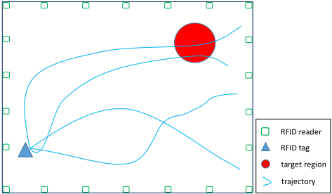
In this section, we formalize the aforementioned setting as an MIL problem. It's natural to regard each trajectory as a bag and the data from different location as instances, and the data collected from the target region is regarded as key instance. In addition, the inconsistencies of data collection result in the problem of key instance shift, which may seriously debase the performance of traditional MIL algorithms and make it necessary to consider the distribution change between training and test phase. In this paper, we apply MIKI to this problem and run experiments to verify its effectiveness.
We sample 80 bags from training data and test data each time, and we collect 30 sets of data in this way. As the results in Table 3 show, MIKI outperforms all other algorithms. The performances of the variants are even worse than miSVM and MILES, verifying again that direct adaptation of importance weighting technique can not work. Moreover, MICS behaves unfavorable, which inspires us that the distribution change of key instances should be addressed.
6 Conclusion
Previous studies of multi-instance learning (MIL) typically assume I.I.D. distribution, which may be violated in many applications. In this paper, we address the problem of MIL with key instance shift and propose an embedding based method MIKI to solve it. Experiments demonstrate the effectiveness of MIKI when key instance shift happens.
We mainly address the key instance shift problem of MIL in this work. We can also consider the scenario that distribution of negative instances varies. More sophisticatedly, distribution of both positive and negative instances may change in some tasks. The success of our proposed methods suggest that it is helpful to make good use of the instances in test bags.
@inproceedings{ijcai2017p481,
  title     = {Multi-Instance Learning with Key Instance Shift},
  author    = {Zhang, Ya-Lin and Zhou, Zhi-Hua},
  booktitle = {Proceedings of the Twenty-Sixth International Joint Conference on
               Artificial Intelligence, {IJCAI-17}},
  publisher = {International Joint Conferences on Artificial Intelligence Organization},
  editor    = {Carles Sierra},
  pages     = {3441--3447},
  year      = {2017},
  month     = {8},
  note      = {Main track},
  doi       = {10.24963/ijcai.2017/481},
  url       = {https://doi.org/10.24963/ijcai.2017/481},
}
TY - CPAPER TI - Multi-Instance Learning with Key Instance Shift AU - Zhang, Ya-Lin AU - Zhou, Zhi-Hua T2 - Proceedings of the Twenty-Sixth International Joint Conference on Artificial Intelligence, IJCAI-17 PB - International Joint Conferences on Artificial Intelligence Organization PY - 2017 SP - 3441 EP - 3447 DO - 10.24963/ijcai.2017/481 UR - https://doi.org/10.24963/ijcai.2017/481 ER -Copied
Machine-readable versions of this paper, for tools and AI agents:





