
SVD-free Convex-Concave Approaches for Nuclear Norm Regularization
Proceedings of the Twenty-Sixth International Joint Conference on Artificial Intelligence. Main track. Pages 3126-3132.
https://doi.org/10.24963/ijcai.2017/436
Keywords
- Machine Learning: Machine Learning
- Constraints and Satisfiability: Solvers and Tools
Abstract
Minimizing a convex function of matrices regularized by the nuclear norm arises in many applications such as collaborative filtering and multi-task learning. In this paper, we study the general setting where the convex function could be non-smooth. When the size of the data matrix, denoted by m x n, is very large, existing optimization methods are inefficient because in each iteration, they need to perform a singular value decomposition (SVD) which takes O(m^2 n) time. To reduce the computation cost, we exploit the dual characterization of the nuclear norm to introduce a convex-concave optimization problem and design a subgradient-based algorithm without performing SVD. In each iteration, the proposed algorithm only computes the largest singular vector, reducing the time complexity from O(m^2 n) to O(mn). To the best of our knowledge, this is the first SVD-free convex optimization approach for nuclear-norm regularized problems that does not rely on the smoothness assumption. Theoretical analysis shows that the proposed algorithm converges at an optimal O(1/\sqrt{T}) rate where T is the number of iterations. We also extend our algorithm to the stochastic case where only stochastic subgradients of the convex function are available and a special case that contains an additional non-smooth regularizer (e.g., L1 norm regularizer). We conduct experiments on robust low-rank matrix approximation and link prediction to demonstrate the efficiency of our algorithms.
- [Abernethy et al., 2009] Jacob Abernethy, Francis Bach, Theodoros Evgeniou, and Jean-Philippe Vert. A new ap- proach to collaborative filtering: Operator estimation with spectral regularization. Journal of Machine Learning Re- search, 10:803-826, 2009.
- [Argyriou et al., 2008] Andreas Argyriou, Theodoros Evge- niou, and Massimiliano Pontil. Convex multi-task feature learning. Machine Learning, 73(3):243-272, 2008.
- [Baccini et al., 1996] Alain Baccini, Ph. Besse, and A. de Falguerolles. A l 1 -norm PCA and a heuristic approach. In Proceedings of the International Conference on Ordinal and Symbolic Data Analysis, pages 359-368, 1996.
- [Cai et al., 2010] Jian-Feng Cai, Emmanuel J Candès, and Zuowei Shen. A singular value thresholding algorithm for matrix completion. SIAM Journal on Optimization, 20(4):1956-1982, 2010.
- [Candès and Recht, 2009] Emmanuel J. Candès and Ben- jamin Recht. Exact matrix completion via convex op- timization. Foundations of Computational Mathematics, 9(6):717-772, 2009.
- [Croux and Filzmoser, 1998] Christophe Croux and Peter Filzmoser. Robust factorization of a data matrix. In Proceedings in Computational Statistics, pages 245-250, 1998.
- [Duchi and Singer, 2009] John Duchi and Yoram Singer. Ef- ficient online and batch learning using forward back- ward splitting. Journal of Machine Learning Research, 10(Dec):2899-2934, 2009.
- [Dudık et al., 2012] Miroslav Dudık, Zaıd Harchaoui, and Jérôme Malick. Lifted coordinate descent for learning with trace-norm regularization. In Proceedings of the 15th International Conference on Artificial Intelligence and Statistics, volume 22, pages 327-336, 2012.
- [Hazan, 2008] Elad Hazan. Sparse approximate solutions to semidefinite programs. In Proceedings of the 8th Latin American Conference on Theoretical Informatics, pages 306-316, 2008.
- [Hsieh and Olsen, 2014] Cho-Jui Hsieh and Peder A Olsen. Nuclear norm minimization via active subspace selection. In Proceedings of The 31st International Conference on Machine Learning, pages 575-583, 2014.
- [Jaggi et al., 2010] Martin Jaggi, Marek Sulovsk, et al. A simple algorithm for nuclear norm regularized problems. In Proceedings of the 27th International Conference on Machine Learning, pages 471-478, 2010.
- [Jaggi, 2013] Martin Jaggi. Revisiting frank-wolfe: Projection-free sparse convex optimization. In Proceed- ings of the 30th International Conference on Machine Learning, pages 427-435, 2013.
- [Ji and Ye, 2009] Shuiwang Ji and Jieping Ye. An acceler- ated gradient method for trace norm minimization. In Pro- ceedings of the 26th Annual International Conference on Machine Learning, pages 457-464, 2009.
- [Ke and Kanade, 2005] Qifa Ke and Takeo Kanade. Robust l 1 norm factorization in the presence of outliers and miss- ing data by alternative convex programming. In Proceed- ings of the IEEE Computer Society Conference on Com- puter Vision and Pattern Recognition, volume 1, pages 739-746, 2005.
- [Lan, 2012] Guanghui Lan. An optimal method for stochas- tic composite optimization. Mathematical Programming, 133:365-397, 2012.
- [Lin et al., 2014] Qihang Lin, Xi Chen, and Javier Peña. A sparsity preserving stochastic gradient methods for sparse regression. Computational Optimization and Applications, 58(2):455-482, 2014.
- [Mahdavi et al., 2012] Mehrdad Mahdavi, Tianbao Yang, Rong Jin, Shenghuo Zhu, and Jinfeng Yi. Stochastic gradi- ent descent with only one projection. In Advances in Neu- ral Information Processing Systems (NIPS), pages 503- 511, 2012.
- [Nemirovski et al., 1982] Arkadi Nemirovski, David Boriso- vich Yudin, and E-R Dawson. Problem complexity and method efficiency in optimization. Wiley-Interscience se- ries in discrete mathematics. Wiley, 1982.
- [Nesterov, 2004] Yurii Nesterov. Introductory lectures on convex optimization: a basic course, volume 87 of Applied optimization. Kluwer Academic Publishers, 2004.
- [Nesterov, 2013] Yu Nesterov. Gradient methods for mini- mizing composite functions. Mathematical Programming, 140(1):125-161, 2013.
- [Pong et al., 2010] Ting Kei Pong, Paul Tseng, Shuiwang Ji, and Jieping Ye. Trace norm regularization: Reformula- tions, algorithms, and multi-task learning. SIAM Journal on Optimization, 20(6):3465-3489, 2010.
- [Rennie and Srebro, 2005] Jasson DM Rennie and Nathan Srebro. Fast maximum margin matrix factorization for col- laborative prediction. In Proceedings of the 22nd Interna- tional Conference on Machine Learning, pages 713-719, 2005.
- [Richard et al., 2012] Emile Richard, Pierre-Andre Savalle, and Nicolas Vayatis. Estimation of simultaneously sparse and low rank matrices. In Proceedings of the 29th Inter- national Conference on Machine Learning, pages 1351- 1358, 2012.
- [Shalev-Shwartz et al., 2011] Shai Shalev-Shwartz, Alon Gonen, and Ohad Shamir. Large-scale convex minimiza- tion with a low-rank constraint. In Proceedings of the 28th International Conference on Machine Learning, pages 329-336, 2011.
- [Signoretto et al., 2013] Marco Signoretto, Volkan Cevher, and JA Suykens. An svd-free approach to a class of struc- tured low rank matrix optimization problems with applica- tion to system identification. In Proceedings of the IEEE Conference on Decision and Control, 2013.
- [Srebro et al., 2005] Nathan Srebro, Jason Rennie, and Tommi S. Jaakkola. Maximum-margin matrix factoriza- tion. In Advances in Neural Information Processing Sys- tems 17, pages 1329-1336, 2005.
- [Toh and Yun, 2010] Kim-Chuan Toh and Sangwoon Yun. An accelerated proximal gradient algorithm for nuclear norm regularized linear least squares problems. Pacific Journal of Optimization, 6(615-640):15, 2010.
References were extracted automatically from the PDF and may contain errors.
Full text extracted automatically from the PDF; figures, tables and equations may differ. The PDF is the version of record.
1 Introduction
Low-rank matrices are preferred in real applications for different reasons. For instance, collaborative filtering uses lowrank matrices to model the fact that preferences of users are limited [Cand`es and Recht, 2009; Abernethy et al., 2009]. Multi-task learning uses low-rank matrices to enforce different tasks to share a common structure [Argyriou et al., 2008; Pong et al., 2010]. To yield low-rank solutions, the following nuclear-norm regularized problems have been widely adopted:
∗Equal Contributions
where f(·) is a convex loss, λ > 0 is a regularization parameter, and ‖A‖∗ = trace(√A⊤A) denotes the nuclear norm of A (i.e., the sum of all the singular values), which is also referred to as the trace norm. Without loss of generality, we assume m ≤ n.
The optimization problem in (1) can be solved by firstorder optimization methods such as subgradient descent [Nesterov, 2004], proximal gradient descent [Duchi and Singer, 2009; Nesterov, 2013]. Although these methods are guaranteed to converge, they are inefficient because a singular value decomposition (SVD), which takes O(m2n) time, is required at each iteration. To reduce the computation complexity, many efficient solvers have been developed by replacing the full SVD with a partial SVD. However, those approaches either require the function f(·) to be smooth [Dudık et al., 2012; Hsieh and Olsen, 2014] or are designed for nuclearnorm constrained problems instead of regularized problems [Jaggi et al., 2010; Jaggi, 2013].
In this paper, we study the general setting of (1), where the function f(·) could be non-smooth, and develop a series of SVD-free optimization algorithms. First, based on the dual characterization of the nuclear norm, we reformulate (1) as a convex-concave optimization problem, and solve it by the subgradient method. In each iteration, we only need to compute the largest singular vector instead of a full SVD, thus reducing the time complexity from O(m2n) to O(mn). As far as we know, this is the first SVD-free convex optimization algorithm for general nuclear-norm regularized problems. Theoretically the proposed algorithm converges at an O(1/√T) rate, which matches the optimal rate of non-smooth optimization under the first-order black-box model [Nesterov, 2004]. Second, we extend our algorithm to stochastic composite optimization, where only stochastic subgradients of f(·) are available, and show that an O(1/√T) rate of convergence is still attainable. Finally, we study the case where an additional non-smooth regularizer such as the ℓ1-norm is presented, and propose a proximal subgradient method that solves the problem at the same rate.
Applications As mentioned above, nuclear norm regularization occurs in many machine learning applications. To motivate this work, we list some applications which involve a convex but non-smooth loss function:
- Robust Low-rank Matrix Approximation: The goal is to fit a target matrix Y with a low-rank matrix A in a robust way [Baccini et al., 1996; Croux and Filzmoser, 1998; Ke and Kanade, 2005]. For this problem, the objective function f(A) = ∑ij |Aij - Yij |/mn, which is non-smooth.
- Sparse and Low-rank Link Prediction: The goal is to discover links from a partially observed adjacency matrix Y such that the link matrix is both sparse and lowrank [Richard et al., 2012]. The objective function is defined as f(A) = ℓ(A, Y ) + γ‖A‖1, where ℓ(A, Y ) is the empirical average of hinge loss over observed entries and thus non-smooth.
2 RelatedWork
In this section, we provide a brief review of existing methods for nuclear-norm regularized problems, as well as related work on nuclear-norm constrained problems.
2.1 Nuclear-normRegularized Problems
Owing to the non-smoothness nature of the nuclear norm, the conventional approach for solving (1) is the subgradient de-
where ∂‖At‖∗ denotes a subgradient of ‖ · ‖∗ evaluated at At, and ηt > 0 is the step size. It is well-known that GD converges to the optimum at an O(1/√T) rate, which is already optimal for first-order optimization of non-smooth functions [Nemirovski et al., 1982; Nesterov, 2004]. When the function f(·) is smooth, proximal gradient descent (PGD), defined as
is preferred and achieves an O(1/T) rate of convergence [Nesterov, 2013]. Following the Nesterov's method for accelerating the gradient method [Nesterov, 2004], an accelerated version of PGD that converges at an O(1/T 2 ) rate has been developed [Ji and Ye, 2009; Toh and Yun, 2010]. Although GD and PGD are guaranteed to converge, they need to calculate the SVD of At or At-ηt∇f(At) in each iteration [Cai et al., 2010], which takes O(m2n) time. Due to the high computational cost of full SVD, GD and PGD do not scale well to large-scale problems.
To reduce the computational complexity, many efficient nuclear norm minimization solvers have been developed. In [Dudık et al., 2012], the authors lift the non-smooth convex problem into an infinitely dimensional smooth problem and apply coordinate descent to solve it. In each round, the algorithm only needs to calculate a partial SVD instead of a full SVD. In [Hsieh and Olsen, 2014], the authors propose the active subset selection (ASS) algorithm, which selects an active subspace by approximating SVD and then cast (1) to a small-size problem that can be solved easily. Although these algorithms are efficient in solving nuclear-norm regularized problem, they are restricted to the case that f(·) is smooth. In contrast, we only assume the function f(·) is convex and it could be non-smooth.
To avoid computing full SVDs, some methods rely on the following variational characterization of the nuclear norm
where the size of the matrices U and V is not constrained. In [Srebro et al., 2005], the authors formulate the problem as semi-define programming and solve it with standard SDP solvers. However, it can not scale up to large datasets. To deal with this limitation, some authors [Rennie and Srebro, 2005; Signoretto et al., 2013] propose alternating direction methods. However, these approaches break the convexity of the original problem and there is no global convergence.
2.2 Nuclear-normConstrained Problems
In [Jaggi et al., 2010], the authors consider a constrained version of (1), i.e.,
They transform it to the problem of optimizing a convex function over the set of positive semi-definite matrices with unit trace, and then use the approximate SDP solver [Hazan, 2008], which in each iteration only calculates an approximate largest eigenvector of the gradient. A similar greedy algorithm has been developed for convex optimization with a low-rank constraint [Shalev-Shwartz et al., 2011]
Recently, the Frank-Wolfe Algorithm has been applied to the nuclear-norm constrained problems [Jaggi, 2013], and also avoids the full SVD operation.
Finally, we note that moving the constraint function into the objective function-a technique utilized in this work, has been leveraged for developing stochastic gradient methods with only one projection [Mahdavi et al., 2012]. However, the differences include (i) we do not need to perform any projection at the end; (ii) their algorithm is to handle the constraint on the primal variable and our algorithm is to handle the constraint on the dual variable.
3 Main Results
In this section, we introduce the details of our SVD-free convex-concave optimization algorithm and several extensions to the basic version.
3.1 The Basic Algorithm
We first recall the dual characterization of the nuclear norm, i.e.,
where ‖U‖2 represents the spectral norm of U. Then, we cast (1) to the following problem
Algorithm 1 SVD-freE CONvex-ConcavE Algorithm (SECONE)
- 1: Initialize: A1 = U1 = 0 ∈ Rm×n
- 2: for t = 1 to T do
- 3: Update At+1 by
- 4: Update Ut+1 by
- 5: end for
- 6: Output: ̂ AT = ∑Tt=1 At/T
Since the above optimization problem is convex-concave, we can apply the standard subgradient method to solve it. However, due to the presence of the spectral norm constraint of U, we have to project the intermediate solution onto the unit spectral norm ball, which again requires a full SVD operation.
To address this issue, we propose to remove the constraint ‖U‖2 ≤ 1, and introduce an additional term into the objective function to control the spectral norm of U:
where ρ > 0 is a parameter whose value will be specified later and [s]+ = max{s, 0} is the hinge operator. To solve the above problem, we can use the standard subgradient method, which iterates as follows:
Note that the subgradient ∂[‖U‖2 - 1]+ can be computed efficiently. To show this, we denote σ1 the leading singular value of U, and u1, v1 the corresponding left and right singular vectors. Then, we have
This implies that in each iteration, we only need to compute the leading singular vectors of Ut with O(mn) time. By contrast, a full SVD takes O(m2n) time. The detailed procedure is summarized in Algorithm 1.
To present the theoretical guarantee of our algorithm, we make the following assumptions of f(·):
Assumption 1. Assume that f(A) ≥ 0 for any A ∈ Rm×n and there exists C > 0 and G > 0 such that f(0) ≤ C and ‖∂f(A)‖F ≤ G. 1
We have the following theorem regarding the optimization error.
Theorem 1. Let ρ ≥ C and run Algorithm 1 with ηt = c1/√t and τt = c2/√t. Let ̂ AT = ∑Tt=1 At/T be the output and U ∗ T = argmax‖U‖2≤1 tr(U ⊤ ̂ AT ). Under Assumption 1 and max{‖At‖F , ‖Ut‖F } ≤ σ, we have
1 To ensure the gradient is bounded, we can add a norm constraint on A if necessary.
The above theorem implies the proposed algorithm has an O(1/√T) convergence rate. And the upper bound is minimized by choosing c1 = D1 √2(G+λσ) and c2 = D2 √2(ρ+λσ) .
3.2 The Stochastic Setting
In this subsection, we extend the basic algorithm to the stochastic setting: f(A) = Eξ[f(A; ξ)], where ξ is a random variable. In this case, the optimization problem becomes
Although existing algorithms for stochastic composite optimization [Lan, 2012; Lin et al., 2014] can be applied to the above problem, they are inefficient because a full SVD operation is required in each iteration.
Following the derivation of (3), we convert the above problem to the unconstrained convex-concave optimization prob-
Generally speaking, it is impossible to compute the gradient of Eξ[f(A; ξ)] w. r. t. A, thus the subgradient algorithm in Algorithm 1 cannot be applied here. Instead, we will first sample a random variable ξt and use the stochastic gradient ∂f(At; ξt) to update the intermediate solution. Specifically, the updating rules are as follows:
The complete procedure is summarized in Algorithm 2.
Before presenting the convergence rate, we make the following assumption.
Assumption 2. Assume that f(A) ≥ 0 for any A ∈ Rm×n and there exists C > 0 and G > 0 such that f(0) ≤ C and Eξ [‖[∂f(A; ξ)]‖2F ] ≤ G2 .
The above assumption requires that the stochastic gradient is bounded in expectation, which is different from Assumption 1 in the deterministic setting. Then, we have the following theorem.
Theorem 2. Let ρ ≥ C and run Algorithm 2 with ηt = c1/√t and τt = c2/√t. Let ̂ AT = ∑Tt=1 At/T be the output and U ∗ T = argmax‖U‖2≤1 tr(U ⊤ ̂ AT ). Under Assumption 2 and max{‖At‖F , ‖U‖F } ≤ σ, we have
where D1 = ‖A∗‖F + σ and D2 = ‖U ∗ T ‖F + σ.
Algorithm 2 Extension to Stochastic Setting (SECONE-S)
- 1: Initialize: A1 = U1 = 0 ∈ Rm×n
- 2: for t = 1 to T do
- 3: Sample ξt
- 4: Update At+1 by
- 5: Update Ut+1 by
- 6: end for
- 7: Output: ̂
The above theorem implies the stochastic version of our algorithm shares the same O(1/√T) rate of convergence with the deterministic version. Given the non-smoothness of the objective function, this rate cannot be improved in general.
3.3 Problems with an Additional Regularizer
In this subsection, we consider the case that besides the nuclear norm regularizer, there is an additional non-smooth regularizer. The optimization problem is given by
where φ(·) is a non-smooth regularizer such as ‖A‖1 and γ > 0 is a regularizer parameter. Note that the proximal gradient descent [Nesterov, 2013] can not be directly applied to (5), because there are two regularizers and there is no closed-form solution to the proximal mapping.
To address this limitation, we propose to solve the following problem
In this way, we only have one regularizer γφ(·), which can be handled by proximal mapping. To be specific, we define the proximal mapping of the convex function h(·) as:
We let h(A) = γφ(A), and introduce the updating rules as:
The detailed procedure is presented in Algorithm 3.
We establish the convergence rate of Algorithm 3 in the following theorem.
Theorem 3. Under the same condition as Theorem 1 and assume φ(0) = 0, we have
where D1 = ‖A∗‖F + σ and D2 = ‖U ∗ T ‖F + σ.
Algorithm 3 Extension to Proximal Variant (SECONE-P)
- 1: Initialize: A1 = U1 = 0 ∈ Rm×n
- 2: for t = 1 to T do
- 3: Update ¯ At+1 by
- 4: Update At+1 by
- 5: Update Ut+1 by
- 6: end for
- 7: Output: ̂
The theorem proves that the proximal variant of our algorithm also converges at an O(1/√T) rate. Though the convergence rate is as same as the one of SECONE, the proximal mapping for ℓ1 norm usually gives us sparse solutions. Also, it is trivial to extend this method to the stochastic optimization algorithm by following the derivation in Section 3.2.
4 Theoretical Analysis
In this section, we provide proofs of Theorems 1 and 3. The proof of Theorem 2 is included in the supplementary.
4.1 Proof of Theorem 1
We start with the unconstrained convex-concave optimization problem (3) by denoting the objective function as
For clarity, we divide the proof into two individual parts.
Part I: Recall that At+1 is the update of subgradient descent applied to L(At, Ut), according to the standard analysis of subgradient descent update, we have for any A ∈ Rm×n
Similarly, Ut+1 is the update of subgradient descent applied to L(At, Ut), hence for any U ∈ Rm×n
With the assumption max{‖At‖F , ‖Ut‖F} ≤ σ and ‖∂f(At)‖F ≤ G, we combine the above inequalities
Let ηt = c1/√t, then simple mathematics shows that
where D1 = ‖A‖ + σ ≥ maxt ‖A - At‖F . We can apply the same analysis for τt = c2/√t and obtain
where we use the fact ∑Tt=1 1 √t ≤ 1 + ∫ T t=1 1 √t dt ≤ 2√T and the notation D2 = ‖U‖F + σ ≥ maxt ‖U - Ut‖F .
Denote that ̂ AT = ∑Tt=1 At/T and ̂ UT = ∑Tt=1 Ut/T. By the convexity of L(A, U) in terms of A and concavity in terms of U, we obtain
To summarize what we have proved, the gap L( ̂ At, U) - L(A, ̂ Ut) decreases at an O(1/√T) rate, which indicates the solution ( ̂ AT , ̂ UT ) converges to the optimal solution of the unconstrained convex-concave optimization problem in (3).
Part II: In the rest of the proof, we will show that the objective value F ( ̂ At) also converges to F(A∗), where A∗ is an optimal solution of the original problem. To see this, we will prove the following inequality
where U ∗ T = argmax‖U‖2≤1 tr(U ⊤ ̂ AT ). First, we have
Thus, it remains to show that
Note that tr(A⊤B) ≤ ‖A‖2‖B‖∗ for any matrices A and B. When ‖̂ UT‖2 ≤ 1, it is easy to verify that (7) holds. In the following, we focus on the case ‖̂ UT ‖2 ≥ 1.
Let ̂ UT have the SVD ̂ UT = PΣQ⊤, where the diagonal matrix Σ = diag(σ1, . . . , σr, σr+1, . . . , σm). The sequence of singular values {σi} is non-increasing and satisfy σr ≥ 1 > σr+1. Denote ˜ UT the projection of ̂ UT onto the unit spectral norm ball. Specifically, it has the form ˜ UT = P ˜ΣQ, where ˜Σ = diag(1, . . . , 1, σr+1, . . . , σm). It follows that
We are now in a position to prove that (7) holds. From Assumption 1, it is easy to verify λ‖A∗‖∗ ≤ C. We have
which is due to the inequality λ‖A∗‖∗ ≤ C and the parameter ρ ≥ C. This completes the proof of Theorem 1.
4.2 Proof of Theorem 3
We may abuse some notations from the previous section. Let L(A, U) = f(A) + λtr(U ⊤A) + γφ(A) - ρ[‖U‖2 - 1]+. Denote that
From the convexity of gt(A) and h(A), we have
From the optimality of At+1 in Algorithm 3, we have
By combining the above two inequality and choosing A = A∗ which is the optimal solution, we obtain
The second inequality follows from Cauchy-Schwartz inequality. Let's consider L(At, Ut) - L(A∗, Ut), which is
Note that the trailing term γ(φ(At) -φ(At+1)) has little impact on the convergence as we assume φ(A1) = φ(0) = 0.
Using the same argument as in the proof of Theorem 1, we can then easily carry out the rest proof of this theorem.
5 Experiments
We present numerical experiments on real datasets to demonstrate the efficiency of the proposed algorithms, and more results can be found in the supplementary.
| Method | c1 | c2 | T | Total CPU time |
|---|---|---|---|---|
| SECONE | 1e7 | 1e4 | 8500 | 6.12e5 |
| PGD | 1e6 | 80 | 6.26e5 | |
| GD | 1e6 | 90 | 6.62e5 |
5.1 Robust Low-rankMatrix Approximation
We consider the robust low-rank approximation problem [Baccini et al., 1996; Croux and Filzmoser, 1998; Ke and Kanade, 2005]:
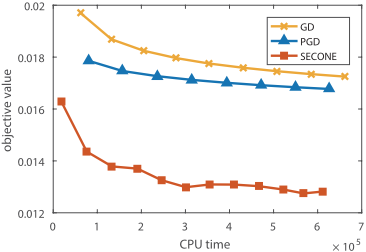
where Y is a given data matrix. Due to the non-smoothness of the objective function, we compare our method with two classical methods: subgradient descent (GD) and proximal subgradient descent (PGD) [Duchi and Singer, 2009]. We use the News20 2 dataset, which contains m = 11, 269 instances, each of which has n = 20, 302 features (we filter the features which appear less than 7 times). According to Theorem 1, we set step sizes in Algorithm 1 as ηt = c1/√t and τt = c2/√t, where c1, c2 are some constants. The same step size ηt = c1/√t is also used for GD and PGD. We tune the value of c1 and c2 in a range of {1e-5, 1e-4, . . . , 1e10} and report the best results based on the objective value.
In Fig. 1, we plot the objective value versus the running time for λ = 1e-6. We choose this value of λ because it can produce a low-rank output, and the convergence behavior is insensitive to λ. As can be seen, SECONE decreases much faster than GD and PGD. This is as expected as SECONE is SVD-free and time-efficient, which is also convinced by the statistics shown in Table 1. As can be seen, each iteration of SECONE takes much less time than other two methods.
5.2 Sparse and Low-rank Link Prediction
Given the adjacency matrix Y of a graph with 0/1 filled entries, we consider the sparse and low-rank link prediction problem:
2 http://qwone.com/˜jason/20Newsgroups/
| Method | c1 or θ | c2 | T | Total CPU time |
|---|---|---|---|---|
| SECONE-P | 1 | 1e-5 | 2000 | 6.43e5 |
| IPD | 0.1 | 50 | 6.57e5 | |
| GD | 1 | 40 | 6.25e5 |
Following the setting in [Richard et al., 2012], we perform experiments on the Facebook100 dataset which contains the friendship relations between students. We select a single university with 41, 554 students and keep the first m = n = 15, 000 users only with the highest degree. We flip 15% of randomly chosen entries and the goal is to learn a sparse and low-rank matrix from the noisy adjacency matrix Y .
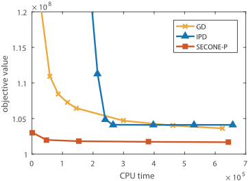
We compare Algorithm 3 (SECONE-P) with subgradient descent (GD) and Incremental Proximal Decent (IPD), which is an iterative algorithm designed for the above problem but with no theoretical guarantees [Richard et al., 2012]. The step sizes in SECONE-P and GD are set in the same way as in Section 5.1. The parameter θ of IPD is searched in the range of {1e-2, 1e-1, . . . , 1e2}.
In Fig. 2, we plot objective value versus the running time when λ = 10 and γ = 0.4. As can be seen, SECONE-P converges much faster than other methods. The tuning of IPD is somewhat tricky since it does not converge to the optimum. The statistics of different methods are shown in Table 2. Again, the running time per iteration of SECONE-P is much smaller than other methods.
Acknowledgments
This work was partially supported by the NSFC (61603177), JiangsuSF (BK20160658), and the Collaborative Innovation Center of Novel Software Technology and Industrialization of Nanjing University. Z. Li and T. Yang are partially supported by National Science Foundation (IIS-1463988, IIS-1545995).
@inproceedings{ijcai2017p436,
  title     = {SVD-free Convex-Concave Approaches for Nuclear Norm Regularization},
  author    = {Xiao, Yichi and Li, Zhe and Yang, Tianbao and Zhang, Lijun},
  booktitle = {Proceedings of the Twenty-Sixth International Joint Conference on
               Artificial Intelligence, {IJCAI-17}},
  publisher = {International Joint Conferences on Artificial Intelligence Organization},
  editor    = {Carles Sierra},
  pages     = {3126--3132},
  year      = {2017},
  month     = {8},
  note      = {Main track},
  doi       = {10.24963/ijcai.2017/436},
  url       = {https://doi.org/10.24963/ijcai.2017/436},
}
TY - CPAPER TI - SVD-free Convex-Concave Approaches for Nuclear Norm Regularization AU - Xiao, Yichi AU - Li, Zhe AU - Yang, Tianbao AU - Zhang, Lijun T2 - Proceedings of the Twenty-Sixth International Joint Conference on Artificial Intelligence, IJCAI-17 PB - International Joint Conferences on Artificial Intelligence Organization PY - 2017 SP - 3126 EP - 3132 DO - 10.24963/ijcai.2017/436 UR - https://doi.org/10.24963/ijcai.2017/436 ER -Copied
Machine-readable versions of this paper, for tools and AI agents:





