
Modeling Trajectories with Recurrent Neural Networks
Proceedings of the Twenty-Sixth International Joint Conference on Artificial Intelligence. Main track. Pages 3083-3090.
https://doi.org/10.24963/ijcai.2017/430
Keywords
- Machine Learning: Deep Learning
- Multidisciplinary Topics and Applications: AI and Ubiquitous Computing Systems
- Uncertainty in AI: Sequential Decision Making
- Machine Learning: Neural Networks
Abstract
Modeling trajectory data is a building block for many smart-mobility initiatives. Existing approaches apply shallow models such as Markov chain and inverse reinforcement learning to model trajectories, which cannot capture the long-term dependencies. On the other hand, deep models such as Recurrent Neural Network (RNN) have demonstrated their strength of modeling variable length sequences. However, directly adopting RNN to model trajectories is not appropriate because of the unique topological constraints faced by trajectories. Motivated by these findings, we design two RNN-based models which can make full advantage of the strength of RNN to capture variable length sequence and meanwhile to address the constraints of topological structure on trajectory modeling. Our experimental study based on real taxi trajectory datasets shows that both of our approaches largely outperform the existing approaches.
- [Cho et al., 2014] Kyunghyun Cho, Bart Van Merriënboer, Caglar Gulcehre, Dzmitry Bahdanau, Fethi Bougares, Hol- ger Schwenk, and Yoshua Bengio. Learning phrase repre- sentations using rnn encoder-decoder for statistical machine translation. arXiv preprint arXiv:1406.1078, 2014.
- [Elman, 1990] Jeffrey L. Elman. Finding structure in time. Cognitive science, 14(2):179-211, 1990.
- [Graves, 2013] Alex Graves. Generating sequences with re- current neural networks. arXiv preprint arXiv:1308.0850, 2013.
- [Gustavsson et al., 2012] Anders Gustavsson, Anders Mag- nuson, Björn Blomberg, Magnus Andersson, Jonas Halfvar- son, and Curt Tysk. On the difficulty of training recurrent neural networks. Computer Science, 52(3):337-345, 2012.
- [Gutmann and Hyvärinen, 2010] Michael Gutmann and Aapo Hyvärinen. Noise-contrastive estimation: A new estimation principle for unnormalized statistical models. In AISTATS'10, pages 297-304, 2010.
- [Hinton, 2012] Geoffrey Hinton. Neural networks for ma- chine learning. Coursera video lectures, 2012.
- [Hochreiter and Schmidhuber, 1997] Sepp Hochreiter and Jürgen Schmidhuber. Long short-term memory. Neural computation, 9(8):1735-1780, 1997.
- [Hochreiter et al., 2001] Sepp Hochreiter, Yoshua Bengio, Paolo Frasconi, and Jürgen Schmidhuber. Gradient flow in recurrent nets: the difficulty of learning long-term depen- dencies, 2001.
- [Jean et al., 2015] Sébastien Jean, Kyunghyun Cho, Roland Memisevic, and Yoshua Bengio. On using very large tar- get vocabulary for neural machine translation. In ACL'15, 2015.
- [Liang et al., 2016] Chen Liang, Jonathan Berant, Quoc Le, Kenneth D Forbus, and Ni Lao. Neural symbolic machines: Learning semantic parsers on freebase with weak supervi- sion. arXiv preprint arXiv:1611.00020, 2016.
- [Maaten and Hinton, 2008] Laurens van der Maaten and Ge- offrey Hinton. Visualizing data using t-SNE. Journal of Machine Learning Research, 9(Nov):2579-2605, 2008.
- [Manning et al., 2008] Christopher D Manning, Prabhakar Raghavan, Hinrich Schütze, et al. Introduction to Infor- mation Retrieval, volume 1. Cambridge University Press, 2008.
- [Mikolov et al., 2013] Tomas Mikolov, Ilya Sutskever, Kai Chen, Gregory S. Corrado, and Jeffrey Dean. Distributed representations of words and phrases and their composi- tionality. In NIPS'13, pages 3111-3119, 2013.
- [Newson and Krumm, 2009] Paul Newson and John Krumm. Hidden markov map matching through noise and sparse- ness. In SIGSPATIAL'09, pages 336-343, 2009.
- [Osogami and Raymond, 2013] Takayuki Osogami and Rudy Raymond. Map matching with inverse reinforcement learn- ing. In IJCAI'13, pages 2547-2553, 2013. IJCAI
- [Ramachandran and Amir, 2007] Deepak Ramachandran and Eyal Amir. Bayesian inverse reinforcement learning. In IJCAI'07, pages 2586-2591, 2007. IJCAI
- [Srivatsa et al., 2013] Mudhakar Srivatsa, Raghu K. Ganti, Jingjing Wang, and Vinay Kolar. Map matching: Facts and myths. In SIGSPATIAL'13, pages 484-487, 2013.
- [Such et al., 2012] Jose M. Such, Agustín Espinosa, Ana García-Fornes, and Carles Sierra. Self-disclosure deci- sion making based on intimacy and privacy. Information Sciences, 211:93-111, 2012.
- [Sundermeyer et al., 2012] Martin Sundermeyer, Ralf Schlüter, and Hermann Ney. LSTM neural networks for language modeling. In INTERSPEECH'12, pages 194-197, 2012.
- [Werbos, 1990] Paul J. Werbos. Backpropagation through time: what it does and how to do it. Proceedings of the IEEE, 78(10):1550-1560, 1990.
- [Wu et al., 2016] Hao Wu, Jiangyun Mao, Weiwei Sun, Bai- hua Zheng, Hanyuan Zhang, Ziyang Chen, and Wei Wang. Probabilistic robust route recovery with spatio-temporal dynamics. In SIGKDD'16, pages 1915-1924, 2016.
- [Xue et al., 2013] Andy Yuan Xue, Rui Zhang, Yu Zheng, Xing Xie, Jin Huang, and Zhenghua Xu. Destination pre- diction by sub-trajectory synthesis and privacy protection against such prediction. In ICDE'13, pages 254-265, 2013.
- [Yuan et al., 2013] Jing Yuan, Yu Zheng, Xing Xie, and Guangzhong Sun. T-drive: Enhancing driving directions with taxi drivers' intelligence. IEEE Transactions on Knowledge and Data Engineering, 25(1):220-232, 2013.
- [Zaremba et al., 2014] Wojciech Zaremba, Ilya Sutskever, and Oriol Vinyals. Recurrent neural network regularization. arXiv preprint arXiv:1409.2329, 2014.
- [Zheng and Ni, 2014] Jiangchuan Zheng and Lionel M. Ni. Modeling heterogeneous routing decisions in trajectories for driving experience learning. In UbiComp'14, pages 951-961, 2014.
- [Ziebart et al., 2008a] Brian D. Ziebart, Andrew L. Maas, J. Andrew Bagnell, and Anind K. Dey. Maximum entropy inverse reinforcement learning. In AAAI'08, volume 8, pages 1433-1438, 2008.
- [Ziebart et al., 2008b] Brian D. Ziebart, Andrew L. Maas, Anind K. Dey, and J. Andrew Bagnell. Navigate like a cab- bie: Probabilistic reasoning from observed context-aware behavior. In UbiComp'08, pages 322-331, 2008.
- [Zimmermann et al., 2016] Max Zimmermann, Eirini Ntoutsi, and Myra Spiliopoulou. Extracting opinionated (sub) features from a stream of product reviews using accu- mulated novelty and internal re-organization. Information Sciences, 329:876-899, 2016.
References were extracted automatically from the PDF and may contain errors.
Full text extracted automatically from the PDF; figures, tables and equations may differ. The PDF is the version of record.
1 Introduction
Cities worldwide seek to make urban living simpler, safer and healthier. Smart mobility is one of the key objectives smart cities want to achieve. In this paper, we focus on trajectory modeling, one of the building blocks for many smart-mobilityrelated initiatives. To be more specific, given a road network (as defined in Definition 1) that captures the roads in a modern city and a trajectory (as defined in Definition 2) recording the movement of a moving object, trajectory modeling is to model the likelihood of a given trajectory with the length k, i.e.,
Definition 1 (Road Network). A road network is modeled as a directed graph G(V, E), where V refers to the set of vertices (i.e., crossroads) and E refers to the set of edges (i.e., road segments). Each edge r ∈ E corresponds to a road segment from a vertex v ∈ V to another vertex v′ (̸= v) ∈ V , where r.s = v /r.e = v′ represent the start/end of the edge.
Definition 2 (Trajectory). A trajectory T in the form of r1 → r2 → · · · → rk captures the movement of an object from r1 to r2 and so on to rk along the road network G, where every two consecutive road segments are connected, i.e., ∀ri, ri+1 ∈ T , ri, ri+1 ∈ E ∧ ri.e = ri+1.s.
Here, P (ri+1|r1:i) is transition probability which captures the probability that a trajectory from r1 to ri takes the segment ri+1, e.g., in front of a traffic light, a driver may have three options, moving straight, turning left, and turning right and probabilities of different options could be very different. It can be regarded as routing decision in the aspect of trajectory, as there might be multiple segments available at the end of ri. We use the notation ra:b to denote the edge sequence from ra to rb (including rb). Note that to simplify the problem, unlike [Such et al., 2012], we define the problem without considering the personality attributes.
Trajectory modeling has a large application base. For example, it can direct self-driving taxis to move along the popular trajectories such that the chance of locating potential commuters is higher; it can enable autonomous vehicles to travel along less popular trajectories in order to relieve traffic congestion; it can help recover the exact trajectory an object moves if the original trajectories are incomplete or uncertain due to low-sampling rate or other reasons; and it can predict the destinations of moving objects in order to have a better estimation of the traffic condition in the near future to ease the planning.
In current literatures, most works use a first-order Markov chain to model the transition probability of trajectory, even though it is known that using Markov chain is not sufficient to model the trajectory [Srivatsa et al., 2013]. To the best of our knowledge, the most relevant work to trajectory modeling lies in the sequential decision literature where a trajectory is modelled by Markov Decision Process (MDP) with the reward function inferred from historical trajectory data using Inverse Reinforcement Learning (IRL). [Zheng and Ni, 2014] and [Ziebart et al., 2008b] are two typical works which adopt IRL techniques to design the model specific to trajectories. However, these models are still too shallow, as MDP adopted by the first work is still a first-order Markov chain and the parameters of the second work are too limited.
On the other hand, it is well-known that Recurrent Neural Networks (RNN) is very powerful in modeling the distribution of sequences with variable length [Graves, 2013]. For example, its Long-Short Term Memory (LSTM) variant can well capture long-term dependency. Unfortunately, we are not able to directly adopt RNN to model trajectory because of the unique constraint trajectories face. Unlike normal sequence (e.g., sentences), trajectories capture the movements from one edge to another while the movement is constrained by the topological structure of road network.
Motivated by above findings, we dedicate this paper to new models that can effectively model trajectories. Our goal is to make full advantage of the power of RNN to capture variable length sequence and meanwhile to address the constraint of topological structure on trajectory modeling. As a summary, we make following two main contributions in this paper. First, to the best of our knowledge, this is the first attempt on adopting deep learning techniques to model road networkconstrained trajectories. We will demonstrate the inefficiency of directly adopting RNN on trajectory modeling via theoretical proof, and propose two new models. Second, we conduct comprehensive experimental study based on real datasets to evaluate the performance and to demonstrate the significant advantages of our new models.
2 RelatedWork
Trajectory models have been adopted to solve many problems in location-based services. [Zheng and Ni, 2014] and [Ziebart et al., 2008b] both implement route recommendation which returns, for a given destination, the trajectory with the highest probability. [Wu et al., 2016] adopts trajectory modeling alike technique to recover the missing portions of a trajectory. [Osogami and Raymond, 2013] uses IRL model to solve map matching problem which is actually a trajectory model extended from [Ziebart et al., 2008a]. Prediction tasks such as [Xue et al., 2013; Yuan et al., 2013] also benefit from trajectory modeling by predicting the probability of road transition.
However, most of these works use a first-order Markov chain to model the transition probability, which is not able to capture the long-term dependencies and meanwhile suffers from sparsity problem [Wu et al., 2016]. Among these works, [Zheng and Ni, 2014] and [Ziebart et al., 2008b] are most relevant to trajectory modeling. Both works solve the problem by recovering the implicit reward through a bunch of historical actions performed by drivers which is similar to finding out the latent features of products from the opinion stream [Zimmermann et al., 2016]. Unfortunately, the first piece of work relies on Bayesian Inverse Reinforcement Learning (BIRL) [Ramachandran and Amir, 2007] that is still based on first-order Markov assumption to model the routing decisions for heterogeneous destinations; the second piece of work adopts Maximum Entropy Inverse Reinforcement Learning (MEIRL) [Ziebart et al., 2008a] and the number of parameters is the dimension of road features, which in turn makes the modeling pattern varieties suffer from too few parameters.
3 RNN for Modeling Sequences
The recurrent neural network [Elman, 1990] is a neural network which can process sequence with arbitrary length. For any time step t, it feeds the input xt and produces the hidden state ht = φ(xt, ht-1) from previous hidden state ht-1, where φ is a non-linear function. By recursively unfolding ht, we will get ht = φ(xt, φ(xt-1, φ(xt-2, φ(...)))) = f (x1:t), indicating that the hidden state of RNN is a function of all past inputs x1:t. By introducing gating mechanism of RNN, e.g., LSTM [Hochreiter and Schmidhuber, 1997] and gated recurrent unit [Cho et al., 2014], which solves the gradient vanishing and exploding problem [Hochreiter et al., 2001], it can be more powerful than shallow sequence models such as Markov chains, and RNNs are popular in modeling language [Graves, 2013; Sundermeyer et al., 2012; Zaremba et al., 2014]. For language modeling task, RNN models the distributions of next word ˜xt+1 given current part of sentence x1:t. At time t, the input is xt. After one iteration in RNN layer, the hidden state of time t (i.e., ht) is produced by φ(xt, ht-1). The output layer adopts a multi-class logistic regression, i.e., an affine transformation with weights W ∈ R|E|×H and biases b ∈ RH followed by softmax function, to get the distribution of the next word. Mathematically,
To adopt RNN in modeling trajectory, we can regard each edge as a word/state and a trajectory as a sentence. However, we want to highlight that the transition from one word to any other word is free, while only the transitions from one edge to its adjacent edges are possible. In other words, the state transition of trajectory is strictly constrained by the topology of road network. Nevertheless, we still can hope RNN to be able to learn the topological constraints and assign close-tozero probabilities to the transitions from one edge ri to any edge rj that is not adjacent to ri. In the following, we will prove that, in order for RNN to achieve above objectives, the number of its hidden units has a lower bound that depends on the state size |E|, the required error and the l2-norm of the weights.
Definition 3 (Legal Transition Set). A legal transition set w.r.t. a vertex v, denoted as S + v , is a set of edges starting from v, i.e, S + v = {r ∈ E|r.s = v} and set S + v contains all the edges that can be legally transited to, from any edge ending with vertex v. Note S - v = E - S + v denotes the illegal transition set w.r.t. v.
For simplicity, we absorb the bias b[i] into the weight vector W [i, :] and denote the new weight as wi. For ht, we omit the subscript t if there is no ambiguity. We use the superscript w+ to denote the weights corresponding to the states in the given legal transition set S + (with subscript v omitted), and w- to denote those in S -. The corresponding sets of weights are referred to as W+ and W- respectively, with W = W+ ∪W-. We use the subscript wmax·h to refer to the weight having the largest inner product with a given hidden state h, i.e., w+max·h = argmaxw∈W+ w⊤h and w-max·h = argmaxw∈W- w⊤h. Moreover, ω denotes the weight having the largest l2-norm, i.e., ω = arg maxw∈W ‖w‖2.
Theorem 1. Given a required error ε and a legal transition set S +, in order to automatically learn the topological structure of the road network G(V,E), i.e., to ensure ∀t the predicted probability of any illegal state is small enough, i.e., smaller than ε |S-| , which in turn holds ∑r∈S- P (r|r1:t) < |S -| × ε |S-| = ε, the lower bound of the number of the hidden units of the last layer (closest to the output layer) an RNN should maintain is [ 1 2‖ω‖2 log (( 1ε - 1)( |E| |S+| - 1))]2 .
Proof. If we want to hold ∀r ∈ S -, P (r|r1:t) < ε |S-| , we should ensure maxr∈S- P (r|r1:t) < ε |S-| , which means
Since the hidden state h of RNN is activated by hyperbolic tangent function, we can ensure, ∀i ≤ H, -1 < h[i] < 1, where H is the dimension of h. Thus ‖h‖2 = √∑Hi=1 h[i]2 < √H. Using the above inequality, we can get,
Adopting triangle inequality, we can get the lower bound of the hidden state dimension, i.e., H, is
4 Our Models: CSSRNN and LPIRNN
According to Theorem 1, it is certain that the lower bound of hidden units of the last hidden layer in traditional RNN with a conventional softmax output is correlated to the state size |E|, the required error ε and the l2-norm of the weights ‖ω‖2. Note that |S +| is always smaller than 6 according to our statistics, which can be regarded as a constant. The expression of the lower bound of H indicates that a larger |E| (city-scale), or a smaller ε, or a smaller ‖ω‖2 (for regularization) will all result in a larger H. Note the above property is not preferable and a larger H will increase the training difficulty of the model with more expensive memory consumption. To overcome the weakness of traditional RNN, we propose two new models, namely CSSRNN and LPIRNN, that are able to incorporate the topological constraints into the model whose hidden units number does not rely on |E|, ε or ‖ω‖2. In addition, since we are not able to use one-hot representation as the input because the number of states is too big, we firstly transform each state into the distributed representation i.e., the dense embedding vector [Mikolov et al., 2013].
4.1 Constrained State Space RNN (CSSRNN)
Our first model CSSRNN is an extension of tradition RNN. As it is hard for the neural network to learn the topology information automatically, we decide to manually feed such information. This idea is similar to [Liang et al., 2016] where the operations necessary for semantic parsing are manually fed instead of learning with a neural network. Here, we choose to input such information in the way of state-constrained softmax function denoted by C(). It replaces the softmax function by only allowing the output of neural network (i.e., the states that current state rt is able to transit to) to go through. In detail, ∀ri ∈ E, we construct a mask vector Mi ∈ R|E| , where
The state-constrained softmax is actually a masked softmax, with a mask dependent on the current state rt. Mathematically,
where ⊙ is the element-wise multiplication. By doing this, the probabilities of the states that cannot be transited from rt will be set to 0 externally. As a result, there is no such lower bound for the number of hidden units to ensure correctly modeling the topological constraints. The additional advantage of setting the transition probabilities of illegal states to zero externally is to allow the model to focus on only updating the weights related to the legal states.
Reducing the computational complexity
Although CSSRNN model addresses the issue of topological constraints, it is still time-consuming as the affine transformation from the hidden state of RNN to the state space, i.e., Wht + b, will still consume O(|E| × H) multiplication and summation operations. Note |E| of a modern city is in the scale of 104 ∼ 105 . In the literature, techniques such as candidate sampling [Jean et al., 2015; Gutmann and Hyv¨arinen, 2010; Mikolov et al., 2013] have been designed to solve the huge state space problem in the domain of NLP. However, those techniques are not preferable to be directly adopted to the state-constrained softmax. On the other hand, we notice that it is not necessary to compute the affine transformation for each state since those corresponding to illegal states will be eventually masked. Accordingly, we introduce a speed-up strategy to train the model to reduce the computational complexity. Since GPU is good at parallelized computation of matrices/vectors, we try to parallel this model to cater for GPU-based training in mini-batch.
To be more specific, we need to construct a legal transition matrix T + and a legal transition mask M+. T + has the dimension of |E| × A, where A = max{|S + v ||S + v ∈ S} and S = {S + v |v ∈ V }. Each row T +[i, :] records all the legal states that ri can transit to. Since the legal transition sets for different states have different sizes, we pad each row with some useless states to standardize the size to A. Next, we construct the corresponding legal transition maskM+ ∈ R|E|×A where M+[i, j ] is set to 0 if T +[i, j ] is a padding state or 1 otherwise. Let b be the batch size, Rt ∈ Rb be the batched input states of t, and Ht ∈ Rb×H be the batched hidden states. Then, the batched distributions of next states can be derived by
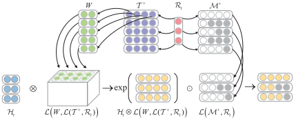
Here, L(P, Q) denotes a look-up operation. It returns an order order(P) - 1 + order(Q) tensor by looking up the first dimension of P according to the elements in Q as the index and tiling these order order(P) - 1 slices in the element order of Q. ∑dim=2 () denotes the summation operation by reducing the second dimension. R = P ⊗Q is a matrix-tensor multiplication operator, where R[i, j ] = ∑k (P [i, k]Q[i, j, k]). Please refer to Figure 1 for a clearer view of the computation flow.
The computation cost for this strategy is, for each sample at each time step, the number of look-up operations is A + 2 and that of summations and multiplications is O(A×H), which makes it independent on the state size |E|. As mentioned before, A is no larger than 6 in most cities based on our study. Compared with the original cost of O(|E| ×H), this strategy significantly reduces the computation cost.
4.2 Latent Prediction Information RNN (LPIRNN)
The second model LPIRNN is constructed by multi-task learning which incorporates the topological information externally using different tasks. In detail, themodel consists of two phases. The first phase is a shared task layer which produces intermediate information, namely latent prediction information, that encodes all the information required by the next task to perform the prediction. The second phase is to perform the prediction by multiple individual tasks. To incorporate the topological constraints, for each input state r, we define an individual model M (η, r) which predicts the distribution of next state within legal transition set S + r.e . The input of the model M(η, r) is the latent prediction information η encoded by the shared task layer. The architecture of this model is shown in Figure 2.
Note that for each individual task model, the state size it needs to predict is very small (no larger than A). If we directly use the output of RNN as the latent prediction, which has the dimension of several hundreds, it might suffer from the curse of dimensionality. Consequently, we add a fully connected layer on the output of RNN to perform automatic dimension reduction. Finally, the distribution of the next legal states w.r.t. current state rt can be written as:
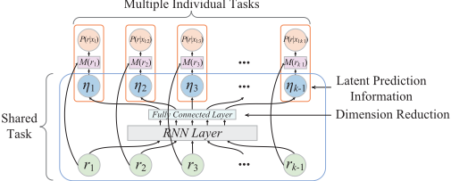
where ηt denotes the latent prediction information produced at time t, F () is a feed forward fully connected layer operation and M () is individual task model handled by a multi-class logistic regression with class number no larger than A.
Explanation of main idea behind LPIRNN
We want the shared task layer to learn certain information satisfying that (1) the strategy to predict such information is homogeneous for all trajectories and (2) it is informative enough to distinguish next state among the states in the legal transition set. For example, the direction information of next road segment satisfies such requirements. The shared task layer predicts the direction information of next road given current part of trajectory, which is a homogeneous task among all input states. For the individual task, given the direction information, it is not hard for a model to predict next road among the legal transition states as they usually have different directions in the real world. By training the whole sequence jointly, i.e, in a multi-task learning way by regarding predicting the probability of one transition (i.e., P (rt|r1:t-1)) as one task, and minimizing each task loss to achieve the minimum loss of the entire trajectory, we believe that the model can learn to predict such homogeneous latent prediction information while fulfilling the heterogeneous prediction tasks. In our experimental study, we will visualize such latent prediction information and study the correlation between this and the direction of roads.
4.3 Difference BetweenCSSRNN and LPIRNN
CSSRNN model has only one weight vector for each to-bepredicted state, i.e., state rj has only one wj regardless of the previous state; while LPIRNN model has one weight for each to-be-predicted state w.r.t. each input state, i.e., rj has a w(rk) rj corresponding to each previous legal state rk (i.e., rk .e = rj.s). Thus, from the parameter view, LPIRNN has more fine-grain weights while CSSRNN defines the weights in a shared way. Intuitively, for a dataset with high density, LPIRNN may perform better than CSSRNN; while for a notsufficient dataset, CSSRNNmay be better. It is also consistent with our experimental results to be presented later.
4.4 Incorporating Destination Information
Given the fact that the destinations of some trajectories are known, we further extend the problem of trajectory modeling. That is to predict a likelihood of a trajectory T for a given destination d.
Both CSSRNN and LPIRNN are flexible to support the above modeling for a given d. We decide to use the distributed representation to feed the destination information. Intuitively, the destination has a big impact on the routing decision. Thus, we claim that if we also train the embedding of the destination during the training of the model, the two destinations d1, d2 embedded to two different roads that are spatially close shall be close as well. In such a way, given d1 or d2 as the destination, the routing decision shall be similar which is also consistent with our everyday experience. We will visualize the trained embedding in the experimental study to justify the above claim. Note that we actually tried to directly input the destination coordinate (with/without normalization), while the result is much poorer than that under the embedding method. We explain the reason may be that the feature size of the coordinate, i.e., 2, is too small, relative to the size of embeddings, e.g., 400 ∼ 600 in our experiment.
4.5 Training
For both models, the goal is to minimize the distribution error between the predicted distribution and the true distribution, thus we adopt the cross-entropy loss as the objective function. Denoting the parameters in RNN as θ, we want to minimize
where 1{condition} is an indicator function and k refers to the length of the trajectory T . The second objective function is for the destination-given trajectory modeling task. As mentioned before, for LPIRNN, we adopt a multi-task learning training style, which means we jointly train the shared task model and individual task model to minimize the cross-entropy loss of the whole sequence. Moreover, E and D refer to the embeddings of input states and destinations states, which will also be jointly trained. The model is trained by employing the derivative of the loss w.r.t. all parameters through backpropagation through time algorithm [Werbos, 1990].
5 Experiment
We use real world taxi GPS trajectory datasets from Porto and Shanghai to conduct the evaluation. The Porto dataset is a 1.8GB open dataset (http://www.kaggle.com/c/pkdd-15-predicttaxi-service-trajectory-i), generated by 442 taxis from Jan. 07, 2013 to Jun. 30, 2014. The Shanghai one is generated by 13,650 taxis from Apr. 01 to Apr. 10 in 2015 with the size of 16GB. We extract the trips occupied by passengers and adopt hidden Markov model based map matching algorithm [Newson and Krumm, 2009] to map the raw GPS sequences to the road networks obtained from OpenStreetMap to generate trajectories. For each city, we extract a large area and a small area. Table 1 reports the statistics of the four datasets.
For each dataset, we evaluate the performances of modeling P (T ) and P (T|d), i.e., model a trajectory without/with destination information. The negative log-likelihood (NLL)
| # Edges | # Vertices | # Trajectories | # Samples per edge | |
|---|---|---|---|---|
| PTlarge | 40,267 | 18,157 | 859,195 | 21.3 |
| PTsmall | 6,117 | 3,182 | 486,268 | 79.5 |
| SHlarge | 60,200 | 28,620 | 3,709,666 | 61.6 |
| SHsmall | 8,075 | 3,632 | 757,032 | 93.8 |
and the prediction accuracy (ACC) are adopted as the performance metrics. NLL is a common metric used by many previous works. ACC computes, the prediction accuracy of next road by the road having the maximum probability. Formally, for a test set with N trajectories,
For the hyperparameter of our models, we split the dataset in the ratio of 8:1:1 to get the training set, validation set and test set. We tune the model according to the validation set and use LSTM [Zaremba et al., 2014] for the RNN layer. For both models, we set the embedding size of input state as 400 for PTsmall and SHsmall, and 600 for SHlarge and PTlarge. We also set the dimension of destination state embedding to be the same as that of input state. We set the hidden unit of LSTM to 400∼600 for different models and the dropout rate for LSTM to be 0.1 using the strategy in [Zaremba et al., 2014]. We train the model using RMSProp algorithm [Hinton, 2012] with a learning rate at 1e-4 and the decay rate at 0.9. We clip the gradient by norm to 1.0 [Gustavsson et al., 2012] and uniformly initialize the embeddings and parameters by [-0.03, 0.03]. For LPIRNN, we set the size of fully connected layer to 200. The source code is available at https://github.com/wuhao5688/RNN-TrajModel.
Baselines
N-gram. We include first, second and third-order Markov chains as the baselines, and we use the conventional name ngram to name them. Laplace smoothing is adopted for sparsity [Manning et al., 2008] which only smooths legal transition states. To model P (T|d), we construct |E| n-grams for each state ri and compute the statistics by the trajectory ending with state ri. BIRL (the model proposed in [Zheng and Ni, 2014] that adopts BIRL [Ramachandran and Amir, 2007]). BIRL does not support the modeling of P (T ) when d is not available. In addition, the training will become extremely slow and hence impractical when the state space is large because of the expensive value/policy iterations with tens of thousands of states. That is the reason why we include two small datasets.
MEIRL (the model proposed in [Ziebart et al., 2008b] which adopts MEIRL [Ziebart et al., 2008a]). Note that MEIRL does not support the modeling of P (T ) as well.
RNN (the sequence model directly adopting traditional RNN [Graves, 2013]). We also use LSTM as the RNN layer with the same embedding and hidden unit size as CSSRNN and LPIRNN.
5.1 Overall Evaluation
The first set of experiments is to evaluate the performance of modeling P (T ) and P (T |d), with the results shown in Table 2. All the approaches achieve better NLL and ACC when the destination is known. This indicates that the routing decision is dependent on the destination which is consist with the expectation. For n-grammodel, it is observed that when the dataset is split by the destination, the performance enhancement w.r.t. the increase of n is limited which indicates that the dataset sparsity occurs and such a memory-based statistics can not handle the task very well. BIRL performs better than n-gram since it takes into consideration the future rewards generated w.r.t. the destination state when modeling the probability to transit to next state. However, it uses MDP which is actually a first-order Markov chain and hence BIRL fails to capture the long term dependency in the past. MEIRL performs not very well, as it models the likelihood of the trajectory based on the maximum entropy criteria, i.e., the likelihood is exponentially proportion to the feature count of the trajectory. It also assumes the feature count is a linear combination of the feature of each state, and hence the parameter of this model is too small (only 20) such that it restricts the representation ability of this model. RNN is a deep model and it can capture the long-term dependency in the past when using LSTM as the RNN layer. Consequently, it outperforms the other shallow models. However, as we have proved that it is hard for traditional RNN to capture the constraints because of the requirements of the size of hidden units, its performance, especially NLL, is far below that of our models. That is to say, traditional RNN tries very hard to predict the distribution rightly but it fails to assign zero probabilities to the illegal states. The performance gap between traditional RNN and our models in the large scale datasets is even more significant than that in the small scale which further justifies our claim.
| Task | Without Destination | With Destination | ||||||||||||||
|---|---|---|---|---|---|---|---|---|---|---|---|---|---|---|---|---|
| Dateset | PTsmall | PTlarge | SHsmall | SHlarge | PTsmall | PTlarge | SHsmall | SHlarge | ||||||||
| Metric | NLL | ACC | NLL | ACC | NLL | ACC | NLL | ACC | NLL | ACC | NLL | ACC | NLL | ACC | NLL | ACC |
| Bi-gram | 8.32 | 90.43% | 9.55 | 90.69% | 9.51 | 83.76% | 9.22 | 85.57% | 6.20 | 94.15% | 8.91 | 92.30% | 7.40 | 88.54% | 7.38 | 89.11% |
| Tri-gram | 7.97 | 90.89% | 9.15 | 91.15% | 9.04 | 84.60% | 8.76 | 86.26% | 6.20 | 93.88% | 8.92 | 91.99% | 7.34 | 87.81% | 7.29 | 88.60% |
| 4-gram | 7.75 | 91.21% | 8.91 | 91.43% | 8.71 | 85.24% | 8.47 | 86.77% | 6.21 | 93.57% | 8.93 | 91.66% | 7.31 | 87.02% | 7.24 | 88.04% |
| BIRL | - | - | - | - | - | - | - | - | 5.84 | 95.53% | - | - | 6.67 | 91.42% | - | - |
| MERIL | - | - | - | - | - | - | - | - | 7.84 | 93.70% | 8.87 | 93.23% | 7.28 | 91.19% | 6.59 | 92.00% |
| RNN | 7.77 | 92.27% | 9.97 | 92.21% | 8.92 | 86.60% | 11.52 | 86.99% | 3.74 | 97.13% | 5.63 | 96.65% | 5.27 | 93.58% | 5.67 | 94.42% |
| CSSRNN | 7.00 | 92.32% | 8.13 | 92.36% | 8.11 | 86.56% | 7.93 | 87.83% | 3.21 | 97.16% | 3.96 | 96.89% | 4.21 | 94.10% | 3.97 | 94.9% |
| LPIRNN | 6.98 | 92.33% | 8.27 | 92.31% | 7.91 | 86.81% | 7.94 | 87.84% | 3.12 | 97.21% | 3.98 | 96.97% | 4.22 | 94.15% | 3.96 | 94.88% |
On the other hand, both CSSRNN and LPIRNN outperform all the competitors with significant advantages. We can observe from the results that LPIRNN performs better than CSSRNN for PTsmall and SHsmall. As both PTsmall and SHsmall have relatively high density according to Table 1, our findings are consistent with the claims made in Section 4.3. When PTlarge that has the lowest density is tested, CSSRNN model which implements the weight sharing strategy outperforms LPIRNN.
5.2 Impacts of the Number of Hidden Units in RNN
We have proved in Theorem 1 that the lower bound of hidden units in the last hidden layer of a traditional RNN is correlated with the required error and the state size. According to that, when the state size is very large (e.g., 104 ∼ 105 for a city), if we want RNN to perform well, we have to increase the number of hidden units in RNN which increases the computation cost and the training difficulty. Here, we conduct the experiments to prove the correctness of the theorem. We adopt the SHlarge dataset since it has the largest state size among the four datasets. Table 3 lists the results, showing that the performance of a traditional RNN greatly reduces with the decreasing of the hidden units. Thus, for an RNN to achieve a good performance given a large size of states, the number of hidden units in the last hidden layer should be increased which justifies our theorem.
| # Hidden units | 50 | 100 | 200 | 400 |
| NLL | 19.90 | 8.04 | 6.90 | 5.27 |
| ACC | 84.38% | 92.24% | 93.55% | 93.58% |
5.3 Impacts of the Initialization Strategy
Since our approach is inspired by the language model and the input of our data is also transformed into the distributed representation, a natural question is that whether pretraining the embedding vectors will enhance the performance of our models. Thus, we conduct the experiments on the initialization of the embeddings. We adopt the well-known word2vec pretraining approach which is often adopted in NLP models [Mikolov et al., 2013]. We use the skip-gram version of the word2vec and set the embedding dimension to 400. We report the NLL and ACC performances of CSSRNN and LPIRNN in Table 4, under the random initialization strategy and the word2vec pretraining strategy respectively. We can find out that using word2vec pretraining strategy to initialize the embeddings of the road segments does not have a significant impact on the performance of both models. This could be caused by the difference between the trajectory data and the natural language. A word in a sentence can be easily changed to another word. For instance, considering the sentence "I'm eating an apple/orange", the pretrained embedding of word "apple" and that of "orange" should be very close via word2vec. This is because in the most situations, these two words are exchangeable which indicates that in the corpus there must be many sentences having the similar contexts of these two words. By pretraining based on the context window, the semantical closeness of words can be modeled. However, for trajectory data, for a given context, the middle road segment in the context is deterministic as road segments have topological constraints. Consequently, in the trajectory data, it is very hard for two road segments having the same/similar contexts, which does not allow context-based pretraining to capture the semantical closeness of road segments. Hence, as a result, we recommend to adopt the randomized initialization strategy.
| Dateset | PTsmall | SHsmall | ||
|---|---|---|---|---|
| Metric | NLL | ACC | NLL | ACC |
| CSSRNN (random) | 3.17 | 97.16% | 4.21 | 94.10% |
| CSSRNN (pretrain) | 3.19 | 97.13% | 4.77 | 93.70% |
| LPIRNN (random) | 3.12 | 97.21% | 4.22 | 94.15% |
| LPIRNN (pretrain) | 3.17 | 97.23% | 4.20 | 94.13% |
| state size | 10K | 20K | 30K | 40K | 50K | 60K |
|---|---|---|---|---|---|---|
| No speed-up (#traj/sec) | 662 | 334 | 221 | 166 | 131 | 109 |
| With speed-up (#traj/sec) | 4563 | 4555 | 4588 | 4556 | 4582 | 4578 |
| Speed-up Ratio | 6.89 | 13.64 | 20.76 | 27.45 | 34.98 | 42.00 |
5.4 The Efficiency of Speed-up Strategy inCSSRNN
Recall that in CSSRNN, we propose a strategy for fast computing the state-constrained softmax function. Table 5 shows the result of with/without this strategy in the forward computation of the model. For the hardware environment, we use one Nvidia GTX 1080 GPU and an Intel Core i7-6700K CPU to run the model. The result demonstrates the efficiency of our speed-up strategy while showing that the computation complexity is irrelevant to the state size.
5.5 Understanding Latent Prediction Information
To have a better understanding of the latent prediction information in LPIRNN, we collect the latent prediction information computed by LPIRNN of all the transition samples that are transited from certain state rt. We adopt Principal Component Analysis (PCA) to reduce the dimensions of the latent prediction information and visualize them. Figure 3(b) plots the result. Each point in the figure represents the latent prediction information w.r.t. an historical transition from the given road rt and the number shown on the point is the next state rt transits to in that sample. We can infer that as discussed in Section 4.2, LPIRNN does predict some latent information like the direction of next road. E.g., road 5924 and road 3670 have totally opposite directions while their latent prediction information is also distant from each other. Meanwhile, roads 2747 and 4373 have the similar directions while in the latent space, they are also close to each other, even though we have not fed the model with any direction information.
5.6 Visualizing the Embedding of Destination
As mentioned in Section 4.4, we adopt the distributed representation to feed destination information and jointly train this embedding when training the model. Here, we visualize the well-trained embedding of destination states using t-SNE [Maaten and Hinton, 2008] algorithm which is popular for reducing the dimension of embedding vectors. Figure 4(b) visualizes some destination embedding corresponding to their road ids. Figure 4(a) shows the location of these roads in the real world. First, we can see, the roads in Figure 4(b), a tiny screenshot in the huge embedding space, are clustered in the embedding space, while they are also close to each other spatially. Second, the relative spatial correlations can also be learned by this embedding, e.g., roads 4823, 4815 and 4819 are close to each other while they are relatively far away from roads 719 and 8054. More interestingly, roads 5713 and 5714 are spatially close but are relatively far away in the embedding space. We then draw the directions of the roads which show that these two roads actually have the opposite directions, which may slightly affect the routing decision, indicating that the model can even learn such information correctly. In conclusion, for trajectory data, using embedding for destination does make sense. The model can perfectly learn certain spatial correlations and directions between states, although we have not fed any spatial and direction information to the model. This is because the routing decision is highly correlated with the position and the direction of destination road and hence the embeddings of spatially close destinations should also be close in order to produce the similar hidden output of the RNN to make the similar routing decisions.
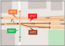
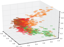
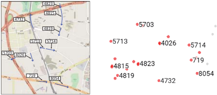
(a) Roads in the map (b) Trained destination embeddings Figure 4: Visualization of the trained destination embeddings.
6 Conclusion
To leverage the strength of RNN to model the sequences and the consideration of trajectories' specific property, we propose two RNN-based models in this paper to model trajectories with/without destination information. The CSSRNN incorporates the topological constraints into the softmax layer and the LPIRNN leverages multi-task learning to address this specific problem. Experiments based on real datasets demonstrate the superiority of our models. Moreover, the visualizations of the result illustrate that our models are able to even learn some interesting spatial and direction information.
Acknowledgments
This research is supported in part by National Natural Science Foundation of China (NSFC) under grant 61073001, Shanghai Natural Science Foundation under grant 14ZR1403100, and the National Research Foundation, Prime Ministers Office, Singapore under its International Research Centres in Singapore Funding Initiative.
@inproceedings{ijcai2017p430,
  title     = {Modeling Trajectories with Recurrent Neural Networks},
  author    = {Wu, Hao and Chen, Ziyang and Sun, Weiwei and Zheng, Baihua and Wang, Wei},
  booktitle = {Proceedings of the Twenty-Sixth International Joint Conference on
               Artificial Intelligence, {IJCAI-17}},
  publisher = {International Joint Conferences on Artificial Intelligence Organization},
  editor    = {Carles Sierra},
  pages     = {3083--3090},
  year      = {2017},
  month     = {8},
  note      = {Main track},
  doi       = {10.24963/ijcai.2017/430},
  url       = {https://doi.org/10.24963/ijcai.2017/430},
}
TY - CPAPER TI - Modeling Trajectories with Recurrent Neural Networks AU - Wu, Hao AU - Chen, Ziyang AU - Sun, Weiwei AU - Zheng, Baihua AU - Wang, Wei T2 - Proceedings of the Twenty-Sixth International Joint Conference on Artificial Intelligence, IJCAI-17 PB - International Joint Conferences on Artificial Intelligence Organization PY - 2017 SP - 3083 EP - 3090 DO - 10.24963/ijcai.2017/430 UR - https://doi.org/10.24963/ijcai.2017/430 ER -Copied
Machine-readable versions of this paper, for tools and AI agents:





