
Locally Consistent Bayesian Network Scores for Multi-Relational Data
Proceedings of the Twenty-Sixth International Joint Conference on Artificial Intelligence. Main track. Pages 2693-2700.
https://doi.org/10.24963/ijcai.2017/375
Keywords
- Machine Learning: Relational Learning
- Machine Learning: Learning Graphical Models
Abstract
An important task for relational learning is Bayesian network (BN) structure learning. A fundamental component of structure learning is a model selection score that measures how well a model fits a dataset. We describe a new method that upgrades for multi-relational databases, a log-linear BN score designed for single-table i.i.d. data. Chickering and Meek showed that for i.i.d. data, standard BN scores are locally consistent, meaning that their maxima converge to an optimal model, that represents the data generating distribution {\em and} contains no redundant edges. Our main theorem establishes that if a model selection score is locally consistent for i.i.d. data, then our upgraded gain function is locally consistent for relational data as well. To our knowledge this is the first consistency result for relational structure learning. A novel aspect of our approach is employing a {\em gain function} that compares two models: a current vs. an alternative BN structure. In contrast, previous approaches employed a score that is a function of a single model only. Empirical evaluation on six benchmark relational databases shows that our gain function is also practically useful: On realistic size data sets, it selects informative BN structures with a better data fit than those selected by baseline single-model scores.
- [Bouckaert, 1995] R. Bouckaert. Bayesian belief networks: from construction to inference. PhD thesis, U. Utrecht, 1995.
- [Buchman and Poole, 2015] David Buchman and David Poole. Representing aggregators in relational probabilistic models. In AAAI, pages 3489-3495, 2015.
- [Chickering and Meek, 2002] David Maxwell Chickering and Christopher Meek. Finding optimal Bayesian net- works. In UAI, pages 94-102, 2002.
- [Domingos and Richardson, 2007] Pedro Domingos and Matthew Richardson. Markov logic: A unifying frame- work for statistical relational learning. In Introduction to Statistical Relational Learning [2007].
- [Frank, 1978] O. Frank. Estimation of the number of con- nected components in a graph by using a sampled sub- graph. Scandinavian Journal of Statistics, pages 177-188, 1978.
- [Friedman et al., 1999] Nir Friedman, Lise Getoor, Daphne Koller, and Avi Pfeffer. Learning probabilistic relational models. In IJCAI, volume 99, pages 1300-1309, 1999. IJCAI
- [Getoor and Taskar, 2007] Lise Getoor and Ben Taskar. In- troduction to Statistical Relational Learning. MIT Press, 2007.
- [Getoor et al., 2001a] Lise Getoor, Benjamin Taskar, and Daphne Koller. Selectivity estimation using probabilistic models. ACM SIGMOD Record, 30(2):461-472, 2001.
- [Getoor et al., 2001b] Lise Getoor Getoor, Nir Friedman, and Benjamin Taskar. Learning probabilistic models of re- lational structure. In ICML, pages 170-177.
- Morgan Kauf- mann, 2001.
- [Getoor, 2001] Lise Getoor. Learning Statistical Models From Relational Data. PhD thesis, Department of Com- puter Science, Stanford University, 2001.
- [Gholami, 2016] Sajjad Gholami. Upgrading Bayesian net- work scores for multi-relational data. Master's thesis, School of Computing Science, Simon Fraser University, 2016.
- [Halpern, 1990] Joseph Y. Halpern. An analysis of first-order logics of probability. Artificial Intelligence, 46(3):311- 350, 1990. IJCAI
- [Kimmig et al., 2014] Angelika Kimmig, Lilyana Mi- halkova, and Lise Getoor. Lifted graphical models: a survey. Machine Learning, pages 1-45, 2014.
- [Laer and de Raedt, 2001] Wim Van Laer and Luc de Raedt. How to upgrade propositional learners to first-order logic: A case study. In Relational Data Mining. Springer Verlag, 2001.
- [Lowd and Domingos, 2007] Daniel Lowd and Pedro Domingos. Efficient weight learning for Markov logic networks. In PKDD, pages 200-211, 2007.
- [Motl and Schulte, 2015] Jan Motl and Oliver Schulte. The CTU prague relational learning repository. CoRR, abs/1511.03086, 2015.
- [Nickel et al., 2016] Maximilian Nickel, Kevin Murphy, Volker Tresp, and Evgeniy Gabrilovich. A review of re- lational machine learning for knowledge graphs. Proceed- ings of the IEEE, 104(1):11-33, 2016.
- [Niu et al., 2011] Feng Niu, Christopher Ré, AnHai Doan, and Jude W. Shavlik. Tuffy: Scaling up statistical infer- ence in markov logic networks using an rdbms. PVLDB, 4(6):373-384, 2011.
- [Pearl, 1988] J. Pearl. Probabilistic Reasoning in Intelligent Systems. Morgan Kaufmann, 1988.
- [Poole, 2003] David Poole. First-order probabilistic infer- ence. In IJCAI, 2003. IJCAI
- [Quinlan and Cameron-Jones, 1993] J. Ross Quinlan and R. Mike Cameron-Jones. Foil: A midterm report. In ECML, volume 667, pages 3-20. Springer, 1993.
- [Russell and Norvig, 2010] Stuart Russell and Peter Norvig. Artificial Intelligence: A Modern Approach. Prentice Hall, 2010.
- [Russell, 2015] Stuart Russell. Unifying logic and probabil- ity. Communications of the ACM, 58(7):88-97, 2015.
- [Sakai and Yamanishi, 2013] Yoshiki Sakai and Kenji Ya- manishi. An NML-based model selection criterion for general relational data modeling. In Big Data, pages 421- 429. IEEE, 2013.
- [Schulte and Gholami, 2016] Oliver Schulte and Sajjad Gho- lami. Consistent bayesian network scores for multi- relational data. StarAI-IJCAI Workshop, July 2016.
- [Schulte and Khosravi, 2012] Oliver Schulte and Hassan Khosravi. Learning graphical models for relational data via lattice search. Machine Learning, 88(3):331-368, 2012.
- [Schulte et al., 2014] Oliver Schulte, Hassan Khosravi, Arthur Kirkpatrick, Tianxiang Gao, and Yuke Zhu. Modelling relational statistics with Bayes nets. Machine Learning, 94:105-125, 2014.
- [Schulte, 2011] Oliver Schulte. A tractable pseudo- likelihood function for Bayes nets applied to relational data. In SIAM SDM, pages 462-473, 2011.
- [Shalizi and Rinaldo, 2013] Cosma Rohilla Shalizi and Alessandro Rinaldo. Consistency under sampling of exponential random graph models. Annals of Statistics, 41(2):508, 2013.
- [Van Haaren et al., 2016] Jan Van Haaren, Guy Van den Broeck, Wannes Meert, and Jesse Davis. Lifted generative learning of Markov logic networks. Machine Learning, 103(1):27-55, 2016.
- [Wang et al., 2008] Daisy Zhe Wang, Eirinaios Michelakis, Minos Garofalakis, and Joseph M Hellerstein. Bayesstore: managing large, uncertain data repositories with proba- bilistic graphical models. In Proceedings VLDB, pages 340-351. VLDB Endowment, 2008.
- [Xiang and Neville, 2011] Rongjing Xiang and Jennifer Neville. Relational learning with one network: An asymp- totic analysis. In AISTATS, pages 779-788, 2011.
References were extracted automatically from the PDF and may contain errors.
Full text extracted automatically from the PDF; figures, tables and equations may differ. The PDF is the version of record.
1 Introduction
Many organizations maintain their data in a multi-relational database. I.i.d. data can be viewed as a special limiting case of multi-relational data with no relationships [Nickel et al., 2016]. Statistical-relational learning (SRL) aims to generalize i.i.d. machine learning methods for multi-relational data; this is called upgrading the method [Getoor and Taskar, 2007; Laer and de Raedt, 2001]. Statistical-relational models have achieved state-of-the-art performance in a number of application domains, such as ontology matching, information extraction, entity resolution, link-based clustering, query optimization, representing uncertainty in databases, etc [Domingos and Richardson, 2007; Niu et al., 2011; Getoor et al., 2001a]. This paper addresses the important SRL task of learning a Bayesian network (BN) structure from a relational dataset.
∗ Supported by a Discovery Grant from the Natural Sciences and Engineering Research Council of Canada. We thank Mark Schmidt and Leonid Chindelevitch for helpful suggestions.
The most common approach to BN structure learning is to search for a structure that optimizes a model selection score for a given dataset. We propose a general method for upgrading BN model selection scores. Our method can be applied with any of the standard BN scores, such as AIC, BIC, BDeu, MDL etc. [Bouckaert, 1995]. Its main theoretical property is preserving local consistency [Chickering and Meek, 2002]: If the i.i.d. model criterion is locally consistent for i.i.d. data, the upgraded criterion is locally consistent for multirelational data. Local consistency combines (i) consistency: as the amount of available data increases, the model selection criterion selects a graph that can represent the data generating distribution, and (ii) optimality: the graph contains no edges that are redundant for representing the data generating distribution. While our theorem generalizes the classic i.i.d. results [Chickering and Meek, 2002], a major point of departure is that we employ a gain function that compares a current vs. an alternative BN structure, rather than a single-model score. The gain function transforms the sufficient statistics for compared structures to the same scale.
Our experiments indicate that the gain function in practice strikes a desirable balance between selecting overly dense and overly sparse structures. In contrast, for baseline scores that are a function of a single model only, the scores either under-weight or over-weight model complexity, selecting either overly dense or overly sparse structures.
Contributions. Our main contributions may be summarized as follows.
- A novel method for upgrading an i.i.d. BN structure score to relational databases, based on a gain function that compares the data fit of two graph structures.
- Preserving local consistency proof: if a score is consistent for i.i.d. data, the upgraded gain function is consistent for relational data. To our knowledge this is the first consistency result for relational structure learning.
Paper Organization. We review background on Bayesian networks and relational data. Then we define our gain function method for upgrading model selection scores, as well as baseline upgrade methods for comparison. Theoretical analysis demonstrates that the gain function method preserves local consistency, whereas the baseline single-model scores do not. Empirical evaluation on six benchmark data sets compares the BN structures selected by the gain function to those selected by the baseline scores, with respect to data fit and model complexity.
2 RelatedWork
Relational Consistency. There have been several recent studies of the consistency of relational learning. Sakai and Yamanishi (2013) provide an asymptotic analysis of selecting the number of relational clusters by optimizing minimum description length. For BN parameter learning, Schulte (2011) upgraded the i.i.d. log-likelihood score by normalizing, which converts feature counts to proportions. Xiang and Neville (2011) prove that the normalized loglikelihood (NLL) is consistent for parameter learning in Markov Logic Networks. We use their framework of learning from one network, to investigate consistency for Bayesian network structure learning. Our gain function extends the NLL score with a normalized model complexity penalty term. The weighted pseudo log-likelihood score for Markov Logic networks [Lowd and Domingos, 2007], also normalizes the log-likelihood term, but not the penalty term, and is nonconsistent for the same reason as the count score defined below.
Consistency and Frequencies. A BN structure G can be parametrized to represent a distribution p if and only if G is an I-map of p, meaning that every d-separation in G corresponds to conditional independence in p [Pearl, 1988]. The blueprint for a consistency argument in the i.i.d. setting is that as the sample size increases, the empirical frequencies approach the data generating distribution p, and the score approaches the maximum likelihood score, and therefore selects an I-map of p. The most straightforward way to generalize this blueprint is to view a multi-relational BN structure as a model of database frequencies, rather than a template model [Getoor, 2001; Schulte et al., 2014]. Using Getoor's terminology, we consider a Statistical-Relational Model (SRM) rather than a Probabilistic-Relational Model (PRM).
Relational Template Models. Many SRL models employ a log-linear likelihood function [Kimmig et al., 2014]; our upgrade method generalizes to any such model. A common approach for defining relational likelihood functions with directed graphical models is to aggregate the information from the multiple parent instances of a ground node using aggregate functions [Getoor et al., 2001b] or combining rules [Poole, 2003]. Recent representation results [Buchman and Poole, 2015] show that such aggregators can be represented in a log-linear model that introduces complex functions (e.g. the number of action movies rated by a user). Since our upgrade method is defined for complex functions, it can in principle be applied to aggregate functions and combining rules. A direct empirical evaluation is currently not possible as there is no implementation of relational BN structure learning with complex functions.
The Inductive Logic Programming FOIL system [Quinlan and Cameron-Jones, 1993] defined the information gain that results from adding a new condition (literal) to a first-order rule. The FOIL information gain is similar to our approach in that 1) it defines a gain function rather than a score, and 2) the key issue concerns adding population variables. It is different in that 1) it is applied with a discriminative not generative model, and 2) different rule groundings are combined using existential quantification rather than a log-linear model.
Previous application of the Learn-and-Join search strategy [Schulte and Khosravi, 2012] used a BN learner for i.i.d. data as a subroutine for learning a multi-relational BN. LAJ search upgrades a BN learning algorithm, but does not define an objective function for model optimization.
3 Background and Notation
We adopt a function-based formalism for combining relational and statistical concepts [Poole, 2003; Russell, 2015]. For a set of random variables X = {X1, . . . ,Xn}, the notation P(X = x) ≡ P(x) denotes the joint probability that each random variable Xi takes on value xi.
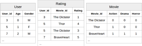
Relational Data A multi-relational model is typically a multi-population model. A population is a set of individuals of the same type (e.g., a set of Users, a set of Movies). Individuals are denoted by constants (e.g., user3 and thor). A k-ary functor, denoted f, f ′ etc., maps a tuple of k individuals to a value. The arguments of a functor are restricted to appropriate types. The possible values of a functor form the domain of the functor. Like [Poole, 2003], we assume that (1) the domain of each functor is finite, and (2) functor values are disjoint from individuals. Throughout the paper we assume complete data. A complete relational dataset or database D, specifies:
- A finite sample population I1, I2 . . ., one for each type.
- The values of each functor, for each input tuple of observed sample individuals of the appropriate type.
Figure 1 shows a toy database. The example follows the closed-world convention: if a relationship between two individuals is not listed, it does not obtain.
Relational Random Variables A population variable ranges over a population, and is denoted in upper case such as User,Movie,A. A term is of the form f(τ1, . . . , τk) where each τi is a population variable or a constant/individual of the appropriate type. A term is ground if it contains only constants; otherwise it is a first-order term with at least one population variable. A first-order random variable (FORV) is a first-order term [Wang et al., 2008]. FORV examples are age(User),rating(User,Movie). We use traditional random variable notation like X, Y for FORVs. 1 A FORV can be instantiated with individual constants, much like an index in a plate model [Kimmig et al., 2014]. A grounding for a list of FORVs simultaneously replaces each population variable in the list by a constant. The number of possible groundings of a joint assignment is given by N [X = x;D] ≡ N [A1;D] × · · · × N [Am;D] where the Ai are the population variables in X and N [A; D] is the size of the sample population of A. The number of satisfying groundings of a joint assignment in database D is denoted by n [X = x; D]. The database frequency [Halpern, 1990] is the number of satisfying groundings over the number of possible groundings:
First-Order Bayesian Networks A Bayesian Network (BN) structure is a directed acyclic graph G (DAG) whose nodes comprise a set of random variables [Pearl, 1988]. A Bayesian network B is a structure G together with a set of parameter values, which specify the distribution of a child node given an assignment of values to its parent node. For an assignment of values to its nodes, a BN defines the joint probability via the standard product formula:
where xi resp. paGi is the assignment of values to node Xi resp. the parents of Xi determined by the assignment x.
A first-order Bayesian network (FOB) [Wang et al., 2008], aka Parametrized BN [Kimmig et al., 2014], is a BN whose nodes are first-order terms. Via Equation (2), a FOB defines a joint distribution over FORVs, so a FOB can be viewed as a Statistical-Relational Model (SRM) of database frequencies [Getoor, 2001]. The semantics of first-order probability logic provides a frequency semantics for FOBs, where a population variable represents an independent random selection from its population [Halpern, 1990; Schulte et al., 2014]. The basis of a model fit score is comparing the joint distribution PB(·) from Equation (2) to the empirical database distribution PD(·) from Equation (1).
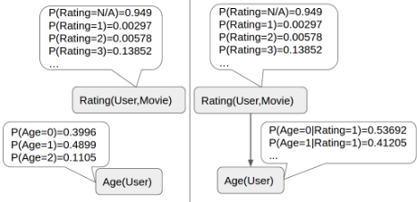
Examples Figure 2 shows an example of two small FOBs. The rating value is n/a (for "not applicable") if and only if the user has not rated the movie (cf. [Russell and Norvig, 2010]). Throughout the paper, conditional probability estimates are computed from the IMDb database described below. Table 1 illustrates database frequencies using the IMDb dataset. The number of users is 941, of which 376 are at age level 0, so the frequency of age 0 users is 376/941. The number of usermovie pairs is 1,582,762 of which 2,524 have the user at age level 0 and a rating of 1. Marginal and joint BN probabilities are computed using Equation (2). The expanded BN B+ 1 matches the database distribution perfectly but at the cost of more parameters.
1 Unfortunately this tradition in statistics clashes with the equally strong tradition in logic of using X, Y for population variables.
| X = x | Age(User) = 0 | Age(User) = 0, Rating (User , Movie ) = 1 |
| n [X = x; D] | 376 | 2,524 |
| N [X = x; D] | 941 | 1,582,762 |
| PD(X = x) | 376/941 ≈ 0.3996 | 2, 524/1, 582, 762 ≈ 0.0016 |
| PB1 (X = x) | 0.3996 | 0.00297 · 0.3996 ≈ 0.0012 |
| PB+ 1 (X = x) | 0.3996 | 0.00297 · 0.53692 ≈ 0.0016 |
4 Multi-Relational Model Comparison
An i.i.d. score measures how well a DAG G fits an i.i.d. dataset D [Chickering and Meek, 2002]. A BN score defines a function S(G, nGijk (D)) that depends on the graph structure and the sufficient statistics nGijk (D). For Bayesian networks, the sufficient statistics are the observed instantiation counts of the possible child-parent configurations. Let Xi = xik,PaGi = paGij be the assignment that sets node i to its k-th value, and its parents to their j-th possible configuration. Then nGijk (D) ≡ n [Xi = xik,PaGi = paGij ;D] is the number of data points that satisfy the ijk assignment. A standard BN score is decomposable, that is, the score can be written as a sum of local scores Si, each of which is a function only of one node Xi and its parents:
We use the following notation for relational sufficient statistics.
- nGijk (D) ≡ n [Xi = xik, PaGi = paGij ; D] is the number of groundings that satisfy the ijk assignment.
- nGij (D) ≡ ∑k nGijk (D) is the number of groundings that satisfy the j-th parent assignment.
- nGi (D) ≡ ∑j ∑k nGijk (D) is the number of possible groundings for node i.
Algorithm 1: The normalized gain method upgrades a decomposable i.i.d. BN score S for multi-relational data.
Input: Database D; Bayesian network DAGs G, G+ where PaGi ⊆ PaG+ i for each node Xi. Output: Gain value ∆S(G, G+, D) Calls local i.i.d. score Si(G, nijk). (Eq. (3))
- 2: for all nodes i do
- 3: ∆Si(G,G+,D) := [Si(G+, nG+ ijk (D)) - Si(G, nGijk (D))]/nG+ i (D) {gain = [score of G+-scaled score of G]/local sample size}
- 4: end for
- 5: return ∑i ∆Si(G,G+,D)
Since the quantity nGi plays the same role as the sample size in i.i.d. data, we refer to it as the local sample size for node i.
We propose a relational gain function ∆S(G,G′ ,D) that measures how much an alternative structure G′ improves a current structure G according to criterion S. Our definition focuses on the case where the alternative G′ adds parents to a node Xi in G. The case where G′ removes parents reverses the role of G and G′ . This is sufficient for applying standard BN structure search algorithms, which consider adding or deleting a single edge at a time, or distinct phases for adding and deleting edges. The gain for edge reversals adds the gains for a deletion and addition. Algorithm 1 shows pseudo code for the gain function. Table 2 gives the normalized gain penalty formulas for upgrading the standard loglikelihood, AIC, and BIC scores [Bouckaert, 1995]. Algorithm 1 can be applied with other scores as well (e.g. for BDeu the normalized gain formula is given in [Gholami, 2016, Section 3.1.3]). We focus on AIC and BIC because they are widely used and have a relatively simple definition.
Motivation Rescaling sufficient statistics for the current graph G (line 1) makes comparable the scores of the current graph and the alternative graph G+. Normalization (line 3) makes comparable the gains for different alternative graphs. The normalization measures the gain per local instance.
Table 3 illustrates the importance of re-scaling counts. The LLi(·, n·ijk (·)) column shows the likelihood score with instantiation counts. This term is an order of magnitude lower for the expanded BN structure G+1 (-2266 vs. -497), simply because the expanded structure increases the local sample size by the number of Movies.
Relationship to Normalized Likelihood In previous work on parameter learning, [Xiang and Neville, 2011; Schulte, 2011], the log-likelihood score LL was upgraded by the normalized log-likelihood score NLL
which converts log-likelihood scores to the same scale, as shown in Table 3. The normalized gain for the log-likelihood score is equivalent to the normalized log-likelihood score differential.
Observation 4.1 The normalized gain equals the difference in normalized log-likelihood. In symbols:
Proof. It suffices to show that LLi(G, nGijk (D))/nG+ i (D) = LLi(G, nGijk (D))/nGi (D). In the scaled log-likelihood LLi(G, nGijk (D)), the scale factor nG+ i (D) nGi (D) does not affect the conditional probability ratio, and can be moved to the front of the sum. Therefore
Many standard BN scores, such as AIC and BIC, are likelihood scores that combine the maximum likelihood of the data under the model with a penalty term f S (#pars G i , nG ijk (D)) that is a function of the number of parameters and the sample size [Bouckaert, 1995]. Observation 4.1 implies that the normalized gain for likelihood scores is equivalent to adding a normalized penalty term to the normalized likelihood. Whereas the normalized likelihood gain can be represented as the difference of two fixed single-model scores, this is no longer true for likelihood scores with penalty terms, because the scaling factor nG+ i (D) is applied to the current graph but depends on the alternative graph. Our evaluation compare the gain function concept with single-model scores as baselines.
Comparison With Single-Model Likelihood Scores. The simplest approach to upgrading an i.i.d. score is to use it with relational instance counts (i.e., Si(G, nGijk (D))). However, this approach has the serious drawback that when a new edge increases the local sample size by connecting different populations, the likelihood decreases while the model complexity increases (see Table 3). Therefore an instance count likelihood score is not consistent, because it fails to add edges that introduce new population variables, no matter how large the sample size (see [Schulte and Gholami, 2016] for empirical confirmation). Our comparison therefore uses likelihood scores that extend the normalized log-likelihood score LL with a penalty term. The count method simply adds the penalty term; the normalized method divides it by the local sample size, which is equivalent to normalizing the instance count score (i.e. Si(G, nGijk (D))/nGi (D)).
Table 4 gives the corresponding formulas for the AIC and BIC penalty terms. Table 5 shows example values for the scores and gains.
| Score S | Si(G+, nG+ ijk (D)) | Si(G, nGijk (D)) | ∆Si(G, G+, D) |
|---|---|---|---|
| LL | ∑j ∑k nG+ ijk (D) · log2 ( nG+ ijk (D) nG+ ij (D) ) | ∑j ∑k nGijk (D) · log2 ( nGijk (D) nGij (D) ) | [LLi(G+, nG+ ijk (D))- LLi(G, nGijk (D))]/nG+ i (D) |
| AIC | LLi(G+, nG+ ijk (D)) - #pars G+ i | LLi(G, nGijk (D)) - #pars G i | ∆LLi(G, G+, D)+ [#pars G i -#pars G+ i ]/nG+ i (D) |
| BIC | LLi(G+, nG+ ijk (D))- log2(nG+ i (D))/2 · #pars G+ i | LLi(G, nGijk (D))- log2(nG+ i (D))/2 · #pars G i | ∆LLi(G, G+, D)+ log2 (nG+ i (D)) 2nG+ i (D) [#pars G i -#pars G+ i ] |
| Family Configuration | nijk | nij | ni | nijk/ni | CP | LLi(·, n·ijk (D)) | LLi(·,n·ijk (D)) nG+ i (D) |
|---|---|---|---|---|---|---|---|
| Age(User)=0 | 376 | - | 941 | 0.3996 | 0.3996 | -497.6217 | -0.5288 |
| Age(User)=0, Rating(User,Movie)=1 | 2524 | 4703 | 1582762 | 0.0016 | 0.5367 | -2266.2224 | -0.0014 |
| Criterion | AICi | BICi |
| Count Score | #pars G i | #pars G i · 1 2 log2 (nG i (D)) |
| Normalized Score | #pars G i nGi (D) | #pars G i · log2 (nG i (D) 2 nG i (D) |
5 Theoretical Consistency Analysis
We formalize consistency for relational data following previous work [Sakai and Yamanishi, 2013; Xiang and Neville, 2011]. The notation N(D) → ∞ from denotes that each population size Ii goes to infinity. Similar to Sakai and Yamanishi, we make the identifiability assumption that
where w represents a complete relational structure (network) from which samples are drawn, and p denotes the generative distribution associated with w. This assumption holds under various sampling schemes such as subgraph sampling [Frank, 1978]. 2 Chickering and Meek introduced the concept of local consistency, which we adapt for gain functions.
Definition 1 Let p be the data generating distribution. A gain function is locally consistent if the following hold as N(D) → ∞, for any graph G and expansion G+ that adds a single edge X+ →Xi to G:
- If X+ is not independent of Xi given PaGi in p, then ∆(G, G+, D) > 0.
- If X+ is independent of Xi given PaGi in p, then ∆(G, G+, D) < 0.
2 Assumptions for consistent parameter learning in PRMs (but not SRMs) are discussed in several papers [Xiang and Neville, 2011; Shalizi and Rinaldo, 2013; Sakai and Yamanishi, 2013].
An upgrade method preserves local consistency if local consistency for an i.i.d. gain function entails local consistency for its upgrade. In the sample size limit, clause 1 entails that the gain of a DAG model is (1) positive for any edge that is necessary for eliminating an independence constraint that does not hold in the generative distribution, and (2) is negative for any edge that is unnecessary. Together, these clauses ensure consistency-necessary edges are learnedand optimality-only necessary edges are learned [Chickering and Meek, 2002].
Theorem 1 The normalized gain upgrade preserves local consistency, and therefore consistency. The single-model comparison scores do not preserve local consistency.
Appendix A gives the local consistency proof for the normalized gain upgrade method. We provide the intuition rather than a formal proof, for why the single-model scores are not locally consistent. The count score fails Clause 1 because neither the NLL nor the parameter count increase with sample size. E.g., if G+1 is correct, its parameter count is 12, whereas the NLL is -1.177 (in Table 5). The penalty term will remain much bigger than the NLL even at large samples fromG+1 .
The normalized score fails Clause 2 because the number of parameters are divided by the local sample sizes. Adding a redundant edge can increase the NLL and decrease the normalized parameter count. For example, the parameter count 12 for G+1 is divided by 1,582,762, whereas the parameter count 2 for G1 is divided by only 941 (Table 5). So even if G1 is optimal, G+1 will receive a higher normalized score even at large samples drawn fromG1. This analysis predicts that the count score selects overly sparse structures, and the normalized score overly dense structures.
| AIC | BIC | ||||||||
|---|---|---|---|---|---|---|---|---|---|
| #groundings | #parameters | LL | count | normalized gain | normalized | count | normalized gain | normalized | |
| G1 | 941 | 2 | -1.384 | -3.38 | - | -1.3865 | -11.26 | - | -1.3948 |
| G+1 | 1582762 | 12 | -1.177 | -13.18 | - | -1.1775 | -124.74 | - | -1.1776 |
| GAIN | 10 | 0.207 | -9.79 | 0.20684 | 0.2090 | -113.48 | 0.20678 | 0.2173 | |
| Dataset | #Relationship Tables/ Total | #Tuples | #Attributes |
|---|---|---|---|
| University | 2 | 171 | 12 |
| Movielens | 1 / 3 | 1,010,051 | 7 |
| Mutagenesis | 2 / 4 | 14,540 | 11 |
| Financial | 3 / 7 | 225,932 | 15 |
| Hepatitis | 3 / 7 | 12,927 | 19 |
| IMDb | 3 / 7 | 1,354,134 | 17 |
6 Empirical Evaluation
Code and Datasets Our code is available on-line. 3 We used six benchmark real-world databases from the CTU Prague Relational Learning Repository, described in [Motl and Schulte, 2015] (also available 4 in text format). Table 6 summarizes basic information about the benchmark datasets. IMDb is the largest dataset in terms of number of total table tuples (more than 1.3M tuples) and schema complexity. It combines the MovieLens database with the Internet Movie Database (IMDb). 5
Model Search Algorithm We used the previous learn-andjoin method (LAJ) for relational BN model search [Schulte and Khosravi, 2012], with the implementation provided by its creators. The LAJ method conducts a search through the lattice of relational paths, similar to the iterative deepening strategy of [Friedman et al., 1999]. At each lattice point, an i.i.d. Bayesian network learner is applied, and learned edges are propagated from shorter paths to longer paths. We reconfigured the LAJ algorithm by changing the score class for each of the 6 upgraded criteria.
Results For each learned graph G, we use maximum likelihood estimates to obtain a Bayesian network B to be evaluated. We report the normalized log-likelihood (NLL) of the input data and the number of parameters for each learned graph. The likelihood is the natural evaluation measure for generative learning [Van Haaren et al., 2016]. Figure 3 shows the metrics for the different upgrade methods.
Count Score. On each dataset, the count score introduces no edges, therefore the smallest number of parameters (for instance 69 on IMDb for AIC count vs. 14,450 for normalized gain). Its NLL metric is substantially worse than the gain NLL on 4/6 databases (e.g. on Financial -12.79 for AIC count vs. -10.79 for the normalized gain). The relatively small absolute difference in NLL on MovieLens and IMDb is due to weak correlations and large local sample sizes. We conclude that the count score structures are overly sparse.
3 github.com/sfu-cl-lab/FactorBase_ Consistent
4 www.cs.sfu.ca/˜oschulte/jbn/
5 grouplens.org, 1M version; IMDb.com, July 2013
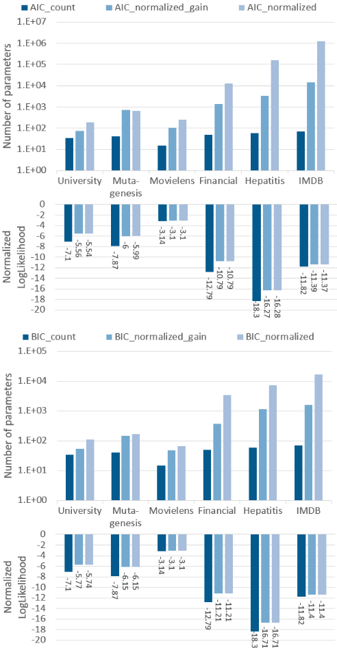
Normalized Score. On each dataset, the normalized score produces the largest number of parameters (for instance 1,199,853 on IMDb for AIC count vs. 14,450 for normalized gain). The normalized gain function achieves almost the same NLL with many fewer parameters. We conclude that the count score structures are overly dense.
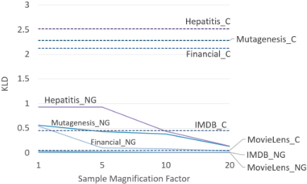
Consistency. The BIC score is consistent for i.i.d. data [Chickering and Meek, 2002], so Theorem 1 entails that the BIC normalized gain is also consistent for relational data. Figure 4 empirically verifies the consistency of the normalized gain criterion, by showing the convergence to the database distribution on our benchmark databases, meaning that the standard Kulback-Leibler divergence (KLD) metric goes to 0. Similar to previous experiments [Getoor et al., 2001a; Schulte et al., 2014], we duplicate entities by a magnification factor of m = 1, 5, 10, 20, which multiplies local sample sizes by m. (We leave out the small University dataset where convergence requires a higher magnification factor.) The BIC count score adds no edges even with larger sample sizes, so it fails to be consistent. The BIC normalized score outputs a denser graph with KLD equivalent to the normalized gain score (Figure 3). So it is consistent but not locally consistent because it selects redundant edges.
7 Conclusion and FutureWork
Generalizing i.i.d. model scores designed for i.i.d. data is an important fundamental topic for relational learning. The normalized gain, which measures the difference in data fit between two BN structures, is a novel scalable method for generalizing a Bayesian network score. For complete data, it can be computed in closed form given the BN sufficient statistics. Normalized gain functions preserve the convergence guarantees of i.i.d. scores, and show good empirical performance: they select structures that succinctly represent the data correlations, compared with baseline single-model scores.
A promising avenue for future work is to apply our approach to other statistical-relational models, such as Markov Logic Networks. Implementing a BN structure learning system for functors that represent complex terms would allow us to apply the normalized gain score with aggregate functions/combining rules.
A Local Consistency Proof for the Normalized Gain Upgrade Method (Theorem 1)
We show the local consistency of the rescaled gain, which is the normalized gain with rescaled sufficient statistics but without dividing by the local sample size:
Since the rescaled gain has the same sign as the normalized gain, proving the local consistency of the rescaled gain implies the local consistency of the normalized gain. We say that an edge adds a population variable if the parent contains a population variable that is not contained in the child.
Case 1: The additional edge X+ → Xi adds no population variables. For such edges, the rescaled counts are the same as the nonscaled counts used in the original i.i.d. score (i.e., nGijk (D) = nGijk (D)). So the arguments of [Chickering and Meek, 2002] can be applied to relational data, and the rescaled gain score is locally consistent in this case.
Case 2: The additional edge X+ → Xi adds a population variable. For concreteness, assume that the edge is of the form g(A, B) → f(A), so the added sample size is N [B; D]. Consider a transformed database D′ where f(A) is replaced by f ′ (A, B), with an inert second argument: f ′ (a, b) = f(a). Since in the transformed schema, the additional edge X+ → X′ i does not add a population variable, from case 1 we conclude that (i) the rescaled gain is locally consistent when applied to the transformed data D′ . We next show that local consistency for D′ data implies local consistency in D data. The transformation does not change the information content and is equivalent to rescaling counts:
Since we also have nG+ ijk (D′ ) = nG+ ijk (D), the transformed and the original data agree on the rescaled gain:
and agree on the conditional probabilities of a child node value given parent node values:
Therefore the identifiability condition (4) for the original data D entails that in the sample size limit, the transformed data D′ identify whether node Xi is independent of X+ given its parents in the data generating distribution p. So by condition (6), the rescaled gain is locally consistent for the original data D. Hence in either case, the normalized gain is locally consistent.
@inproceedings{ijcai2017p375,
  title     = {Locally Consistent Bayesian Network Scores for Multi-Relational Data},
  author    = {Schulte, Oliver and Gholami, Sajjad},
  booktitle = {Proceedings of the Twenty-Sixth International Joint Conference on
               Artificial Intelligence, {IJCAI-17}},
  publisher = {International Joint Conferences on Artificial Intelligence Organization},
  editor    = {Carles Sierra},
  pages     = {2693--2700},
  year      = {2017},
  month     = {8},
  note      = {Main track},
  doi       = {10.24963/ijcai.2017/375},
  url       = {https://doi.org/10.24963/ijcai.2017/375},
}
TY - CPAPER TI - Locally Consistent Bayesian Network Scores for Multi-Relational Data AU - Schulte, Oliver AU - Gholami, Sajjad T2 - Proceedings of the Twenty-Sixth International Joint Conference on Artificial Intelligence, IJCAI-17 PB - International Joint Conferences on Artificial Intelligence Organization PY - 2017 SP - 2693 EP - 2700 DO - 10.24963/ijcai.2017/375 UR - https://doi.org/10.24963/ijcai.2017/375 ER -Copied
Machine-readable versions of this paper, for tools and AI agents:





