
Distributed Accelerated Proximal Coordinate Gradient Methods
Proceedings of the Twenty-Sixth International Joint Conference on Artificial Intelligence. Main track. Pages 2655-2661.
https://doi.org/10.24963/ijcai.2017/370
Keywords
- Machine Learning: Machine Learning
- Machine Learning: Classification
Abstract
We develop a general accelerated proximal coordinate descent algorithm in distributed settings (Dis- APCG) for the optimization problem that minimizes the sum of two convex functions: the first part f is smooth with a gradient oracle, and the other one Ψ is separable with respect to blocks of coordinate and has a simple known structure (e.g., L1 norm). Our algorithm gets new accelerated convergence rate in the case that f is strongly con- vex by making use of modern parallel structures, and includes previous non-strongly case as a special case. We further present efficient implementations to avoid full-dimensional operations in each step, significantly reducing the computation cost. Experiments on the regularized empirical risk minimization problem demonstrate the effectiveness of our algorithm and match our theoretical findings.
- [Bradley et al., 2011] Joseph Bradley, Aapo Kyrola, Danny Bickson, and Carlos Guestrin. Parallel coordinate descent for l1-regularized loss minimization. ICML, 2011.
- [Dunner et al., 2016] Celestine Dunner, Simone Forte, Mar- tin Takac, and Martin Jaggi. Primal-dual rates and certifi- cates. ICML, 2016.
- [Fan and Lin, 2011] Rong-En Fan and Chih-Jen Lin. Lib- svm data: Classification, regression and multi-label. URL: http://www.csie.ntu.edu.tw/ cjlin/libsvmtools/datasets, 2011. Link
- [Fercoq and Richtarik, 2015] Olivier Fercoq and Peter Richtarik. Accelerated, parallel and proximal coordinate descent. SIAM Journal on Optimization, 2015.
- [Lin et al., 2014] Qihang Lin, Zhaosong Lu, and Lin Xiao. An accelerated proximal coordinate gradient method and its application to regularized empirical risk minimization. NIPS, 2014.
- [Ma et al., 2015] Chenxin Ma, Virginia Smith, Martin Jaggi, Michael Jordan, Peter Richtarik, and Martin Takac. Adding vs. averaging in distributed primal-dual optimiza- tion. ICML, 2015.
- [Necoara and Clipici, 2013] Ion Necoara and Dragos Clipici. Efficient parallel coordinate descent algorithm for convex optimization problems with separable constraints: application to distributed mpc. Journal of Process Control, 2013.
- [Nesterov, 1983] Yurii Nesterov. A method of solving a con- vex programming problem with convergence rate o(1/k 2). Soviet Mathematics Doklady, 1983.
- [Nesterov, 2012] Yurii Nesterov. Efficiency of coordinate de- scent methods on huge-scale optimization problems. SIAM Journal on Optimization, 2012.
- [Richtarik and Takac, 2013a] Peter Richtarik and Martin Takac. Distributed coordinate descent method for learn- ing with big data. arXiv:1310.2059, 2013.
- [Richtarik and Takac, 2013b] Peter Richtarik and Martin Takac. Parallel coordinate descent methods for big data optimization. arXiv:1212.0873v2, 2013.
- [Shalev-Shwartz and Zhang, 2014] Shai Shalev-Shwartz and Tong Zhang. Accelerated proximal stochastic dual coorid- inate ascent for regularized loss minimization. ICML, 2014.
- [Takac and Richtarik, 2015] Martin Takac and Pe- ter Richtarik. Distributed mini-batch sdca. arXiv:1507.08322v1, 2015.
- [Wright, 2015] Stephen Wright. Coordinate descent algo- rithms. Mathematical Programming 151.1, 3-34., 2015.
- [Xiao and Lu, 2013] Lin Xiao and Zhaosong Lu. On the complexity analysis of randomized block-coordinate de- scent methods. arXiv:1304.4723, 2013.
- [Yang, 2013] Tianbao Yang. Trading computation for com- munication: Distributed stochastic dual coordinate ascent. NIPS, 2013.
References were extracted automatically from the PDF and may contain errors.
Full text extracted automatically from the PDF; figures, tables and equations may differ. The PDF is the version of record.
1 Introduction
We consider the following optimization problem with a composite objective function:
where f and Ψ are proper and lower semi-continuous convex functions. We further assume that f is differentiable on RN , and Ψ has a simple blockwise separable structure Ψ(x) = ∑ni=1 Ψi(xi), where xi is the i-th block of x with cardinality Ni. This problem is ubiquitous in machine learning, where f(x) denotes the loss and Ψ represents some constraints or regularizations. Given a set D of i.i.d data, a typical loss function f has the following form
where l is some smoothed loss function such as the smoothed hinge loss [Lin et al., 2014]. The choice of Ψ depends on the requirements of certain problems, such as bound constraints (e.g., Ψi(x) = 0 for x ∈ [0, 1] and ∞ otherwise) or regularizations for a special purpose (e.g., L1-regularizer for sparsity). f(x) can be strongly convex or not. The strong convexity property usually means a faster (linear) convergence rate and hence is interested in many cases (e.g., ridge regression). We aim to develop a general accelerated coordinate descent method to solve problem (1) under distributed settings, and accelerate the convergence rate by making use of the parallel structure.
∗Corresponding author
1.1 RelatedWork andMotivation
Coordinate descent (CD) methods are popular optimization algorithms to handle such problems that can break down to small pieces since they can usually make use of special structures underlying the problems. At each iteration t, the basic CD method chooses one block of coordinate xit to sufficiently reduce the objective value while keeping the other blocks fixed. There are two common strategies for choosing such a block-the cyclic scheme and the randomized scheme, where the former chooses it in a cyclic fashion (i.e., it+1 = it mod n + 1), while the latter chooses it uniformly or via some distributions. The randomized scheme is more common since it enjoys both theoretical and practical benefits [Wright, 2015]. Due to their superior convergence property, CD algorithms have been widely used in many practical problems, especially in some regimes that need relatively high accurate solutions [Wright, 2015].
To improve the performance of the basic CD algorithm, many variants have been proposed. Among them, Nesterov's acceleration technique [Nesterov, 1983], which is proven to be an "optimal" first order (gradient) method in convergence rate, is an important line. Specially, Nesterov [2012] developed an accelerated randomized CD method for minimizing unconstrained smooth functions (i.e., with Ψ(x) = 0), which is the first one that applies acceleration techniques to CD methods. Later one, Lu and Xiao [2013] gave an improved version with a sharper convergence analysis. For the more general problem (1), Fercoq and Richtarik [2015] proposed the APPROX algorithm for solving functions f(x) without strong convexity to obtain an accelerated sublinear convergence rate and Lin [2014] proposed a general APCG algorithm to obtain an accelerated convergence rate for f(x) either with strong convexity or not.
Another important line is to utilize parallel computing architectures to accelerate the CD algorithms. Here we focus on the synchronous case, where multiple blocks of coordinates are sampled and gradients are then computed in each iteration, running in parallel on multiple processors. After that, a barrier synchronization step is set to update the coordinates, see a series of recent work in parallel and distributed settings [Bradley et al., 2011; Necoara and Clipici, 2013; Richtarik and Takac, 2013a]. To meet the requirements of the big-data challenge, combining the acceleration technique with advanced parallel computing architectures seems to be natural to leverage their advantages respectively. For the general problem (1), the APPROX algorithm is parallel in nature to deal with f(x) without strong convexity. For a special case of (1) called empirical risk minimization (ERM) problem, Shalev-Shwartz and Zhang [2014] proposed an innerouter loop optimization scheme to obtain an accelerated convergence rate with a strong convexity assumption, where the inner loop is easily parallelized using existing techniques [Takac and Richtarik, 2015]. However, the parallel algorithm for problem (1) in the strongly convex case is still unexplored.
In this paper, we propose a new distributed accelerated coordinate gradient descent method (DisAPCG) to solve the general form (1) for f(x) with or without strong convexity. Our algorithm lies in the line of Nesterov acceleration methods, with new carefully modified Nesterov's sequences to adapt into distributed settings. Our algorithm includes APPROX as a special case when the function does not have a strong convexity assumption, where a sublinear convergence rate is obtained. In the strong convex case, we obtain an accelerated linear convergence rate, thanks to the parallel structure. Furthermore, we propose an efficient implementation to avoid full-dimensional vector operations, which reduces the updating cost in each iteration. For practical use, we apply our algorithm to the ERM problem and find a significant improvement comparing with several other distributed CD solvers.
1.2 Outline of The Paper
In Section 2, we introduce the notations and assumptions, present the general DisAPCG method, analyze its convergence rate with or without strong convexity, and show the gain by leveraging parallel structures. In Section 3, we present an equivalent version of the general algorithm to avoid full-dimensional manipulation in many cases. In Section 4, we apply our DisAPCG method to the widely studied ERM problem. Besides, we use experiments on a smoothed version of SVM problems to demonstrate the effectiveness of our algorithm. Finally, we conclude in Section 5.
2 The DisAPCGMethod
2.1 Notations, Assumptions and Settings
For an N-dimensional vector x ∈ RN , let Ω = {xi ∈ RNi }ni=1 denote a partition of the coordinates with ∑ni=1 Ni = N. Let U = [U1, ..., Un] be an N × N permutation matrix with Ui ∈ RN×Ni . Then, we have
Without losing generality, we assume that U is the identity matrix. Our distributed setting is similar as in [Richtarik and Takac, 2013a]. Suppose that the cluster consists of K nodes and the blocks of coordinates (features) are uniformly distributed in each node (i.e., each node keeps and updates n/K blocks of coordinates). For simplicity, we assume that n is divisible by K. We denote Sk ⊂ Ω as the collection of blocks of coordinates that are distributed in the k-th node and we have ∪Kk=1Sk = Ω. In the meanwhile, all the data describing the features Sk are stored in the k-th node.
Following [Lin et al., 2014], for any x ∈ RN , the partial gradient of f with respect to xi is defined as
where [n] := {1, ...n} denotes the set of integers from 1 to n. We make the following assumptions, which are commonly used in the literature of coordinate descent methods [Fercoq and Richtarik, 2015].
Assumption 1. The gradient of f(x) is block-wise Lipschitz continuous with constants Li:
the L2-norm blockwisely weighted by the coefficients Li.
Assumption 2. There exists µ ≥ 0 such that for all y ∈ RN and x ∈ dom(Ψ):
An immediate consequence of Assumption 1 is
which bounds the variation of f(x) when a single block changes. In distributed settings, as more than one blocks vary in each iteration, we need the following lemma to bound the total variation of the function f(x).
Lemma 1. ([Richtarik and Takac, 2013b]) Assume that f satisfies Assumption 1. For all x, h ∈ RN , we have
where Supp(h) := {i ∈ [n] : h(i) ̸= 0} is the set of blocks that are not equal to zero.
The above bound is tight in general. Suppose that in distributed settings, we alter κ blocks in each iteration and define
∥ · ∥2Lκ = κ∥ · ∥2L.
and Assumption 1 implies that
2.2 The DisAPCGAlgorithm
The general DisAPCG algorithm is summarized in Alg.1. We start K processors and each processor k runs Alg.1 simultaneously. The algorithm maintains a non-increasing step size αt and intermediate variable y(t) , similarly in the original Nesterov's method. At iteration t, each node samples multiple blocks of coordinates and computes the intermediate variable z(t) using a proximal gradient step, as in step 4. Finally,
the coordinates are updated in a synchronized manner in step 5. We make more comments on several key steps as follows.
Step1: S(t) k collects the indices of the coordinates to be updated for node k. The total number of updated coordinates in one iteration is κ = τK, where τ is the mini-batch size that every node samples at each iteration. Note that the sample procedure is not equivalent to uniformly sample κ blocks of coordinates from all since they are stored locally.
Our algorithm is essentially in a mini-batch manner. When K = 1, we can merge several small blocks into a larger one and use [Lin et al., 2014] directly (i.e., uniformly sample one large block at each iteration), and hence the mini-batch analysis is not necessary. However, such merging can not be done in the distributed settings, since every node needs to sample their own data, not as a whole.
Step2: The original Nesterov's sequence is computed as n2α2 t = (1 - αt)γt + αtµ. Our new sequence considers the influence introduced by multi-block alteration in one iteration. Similar properties hold as the original ones.
Step3: The Reduce operator is similar to MPI::AllReduce, where y(t) is first computed by gathering coordinates from all nodes and then broadcasted to all nodes. This is a crucial step since y(t) is of size O(N) and hence introduces the most part of communication cost. y(t) is used to compute the gradient, however, one can further reduce the communication cost by exploring the special structure of f(x), as we shall see.
Step5: The update step involves full-dimensional operations since z(t+1) , z(t) and y(t) are dense in general and the similar problem exists for the computation of y(t) . This issue will be dealt with by proposing an efficient and equivalent algorithm in Section 3.
2.3 Convergence Analysis
We analyze the convergence rate of Alg.1. The main theorem is as follows. We defer the full proof into appendix.
Theorem 1. Suppose that Assumptions 1 and 2 hold. Let F ∗ be the optimal value of problem (1) and {x(t) } be the sequence generated by the DisAPCG method. Then for any t ≥ 0, the following holds:
where R0 := min x∗∈X∗ ∥x(0) - x∗ ∥2L, and X∗ is the set of optimal solutions of problem (1).
respond to the strong convex and non-strong convex cases respectively. For the non-strongly convex case, a slight change of the proof can remove the κ in the last term of (7) and then we recover the convergence rate in [Fercoq and Richtarik, 2015] as a special case.
For the strongly convex case, we get an accelerated linear convergence rate, as the following corollary shows:
Algorithm 1 The DisAPCG algorithm.
Input: x(0) ∈ dom(Ψ) and convexity parameter µκ ≥ 0. Initialize: set z(0) = x(0) and choose 0 < γ0 ∈ [µκ, 1]. Start K nodes with their corresponding data and coordinates. for t = 0, 1, 2, 3... do:
- Uniformly sample τ blocks of coordinates S(t) k .
- Compute αt ∈ (0, κ/n] using the relation:
- for all index i ∈ Sk, compute z(t+1) i as
and for all index i ̸∈ Sk, compute z(t+1) i as
end for
Corollary 1. Suppose that the same conditions in Theorem. 1 hold and further assume that f is µ-strongly convex. In order to obtain E[F(x(t) ] -F ∗ ≤ ϵ, it suffices to have the iteration t satisfy
The previous single-machine version APCG provided in [Lin et al., 2014] needs O(n/√µ) to achieve ϵ accuracy, while our DisAPCG further accelerates this rate by a factor √κ, omitting the log term. It remains an open problem that whether we can accelerate this rate by κ.
Remark 1. We have assumed that the coordinates (and their corresponding data) are uniformly distributed in each node. However, the computation power of each node may be different in practice, in which stragglers may slow down the barrier synchronization. To avoid this, nodes can store different amounts of coordinates, depending their computation power, and consequently, each node k has its own mini-batch size τk. The above theorem still holds as long as each block is sampled with equal probability.
3 Efficient Implementation
For the strongly convex case with µ > 0, we can choose γ0 = µ/κ to get a concise version. In this case, we have that γt = µ/κ and consequently, αt = βt = √κµ/n.
As mentioned in Section 2.2, a straightforward implementation of Alg.1 requires full-dimensional operations on x (i.e. O(N)), which is comparable to a full-gradient step. Lin et al. [2014] provided an equivalent version to their original algorithm, corresponding to the special single-machine case in our paper, with an efficient update step. Here we show that such strategy can also be used in the distributed settings with some modifications. The overall algorithm is summerized in Alg.2 and the equivalent assertion is made in Proposition 1. Proof can be found in the appendix.
Algorithm 2 DisAPCG without full-dimensional vector operators in the case µκ > 0
Input: x(0) ∈ dom(Ψ) and convexity parameter µκ > 0. Initialize: set u(0) = 0, v(0) = x(0) , α = √κµ n , ρ = 1-α 1+α . Start K nodes with their corresponding data and coordinates. for t = 0, 1, 2, 3... do:
- Reduce: ρt+1u(t) + v(t) .
- Uniformly sample τ blocks of coordinates S(t) k .
- for all i ∈ S(t) k compute h(t) i as
Output: x(t) = ρtu(t) + v(t) .
Proposition 1. Algorithm 2 and Algorithm 1 are equivalent with
for all t ≥ 0.
As we can see, the updating step in Alg.2 avoids fulldimensional operations. However, the reduce step ρt+1u(t) + v(t) still needs O(N) computation cost in general. We can further explore the structure of certain problem to avoid it, as we shall see for the problem of ERM.
4 Application to Primal-dual ERMProblem
4.1 Primal and Dual ERMProblem
The ERM problem arises ubiquitously in supervised machine learning applications. Let A1, ...,An be vectors in Rd , ϕ1, ..., ϕn be a sequence of convex functions on R, and g be a convex function on Rd , the regularized ERM problem is defined as follows:
The dual of the above problem is
where A = [A1, ...,An], and ϕ∗ , g∗ are conjugate functions of ϕ, g respectively.
Notice that in the above problem, the sample size n is the dimensionality when we consider the dual problem. We focus on the strong convexity case, where we need the following assumption that is also standard in the literature of solving the primal and dual ERM problems.
Assumption 3. Each function ϕi is 1/γ smooth and the function g is strong convex with parameter 1.
The above assumption implies that ϕ∗i is γ strong convex and g∗ is continuous differentiable.
The structure of D(x) matches problem (1) with the equivalent form F(x) = -D(x), where f(x) = λg∗ ( 1 λn Ax)
and Ψ(x) = 1n ∑ni=1 ϕ∗i (-xi). In order to match the linear convergence rate assumption, we re-locate the strong convexity of ϕ∗i and get the final optimization problem as argminx∈Rn F (x) where
We focus on a special case that g(w) = 12 ∥w∥22 . Such special case implies that we can efficiently compute the partial coordinate gradient and is mostly used as regularization term in ERM problems [Ma et al., 2015]. In this case, we have
Besides, we can determine an upper bound for the Lipschitz constant Li ≤ R2 + λγn λn2 , where R = max∥Ai∥2, i ∈ [n], and a lower bound for the strong convexity parameter for f(x) with respect to ∥ · ∥L as µ ≥ λγn R2 + λγn . Details can be found in the appendix.
4.2 Numerical Experiments
We consider minimizing the smoothed hinge loss problem, in order to satisfy the 1/γ smooth condition. Precisely, we have
The conjugate function of ϕi is then as follows:
Consequencely, we have
In the context of primal-dual optimization problem, people often care about the duality gap P(w(x)) -D(x), which is Algorithm 3 DisAPCG for regularized ERM with µ > 0
Start K nodes with their corresponding data and coordinates. for t = 0, 1, 2, 3... do:
- Reduce: p(t) , q(t) .
- Uniformly sample τ blocks of coordinates S(t) k .
- for all i ∈ S(t) , compute:
Output: primal and dual solutions:
| datasets | dimension d | sample size n | sparsity |
|---|---|---|---|
| epsilon | 2,000 | 100,000 | 100% |
| covtype | 54 | 581,012 | 22% |
| RCV1 | 47,236 | 677,399 | 0.16% |
an upper bound to the gap D∗ -D(x). An overall discussion about the relation between these gaps can be found in [Dunner et al., 2016]. Here we directly use the duality gap as the statistical indicator.
We implement the algorithms by C++ and openMPI and run them in clusters on Tianhe-II super computer, where in each node we use a single cpu. Experiments are performed on 3 datasets from [Fan and Lin, 2011] whose information is summarized in Table 1.
Influence of mini-batch size τ and number of nodes K
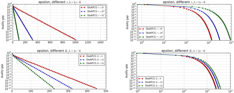
We first analyze the influence of the mini-batch size τ and the number of nodes K on the Epsilon dataset. We either vary the mini-batch size τ on each node with the number of nodes K fixed, or vise versa. Intuitively, a larger mini-batch size τ means a larger descent in one iteration, however, it needs more computation cost. Similarly, a larger number of nodes K means a larger descent while more communication cost. Therefore, on the one hand, we show the duality gap w.r.t the number of iterations to verify the linear convergence rate and the benefits by increasing computation resources. On the other hand, we show the duality gap w.r.t running time to make clear the trade-off between computation and communication.
The overall results are summarized in Fig.1. In terms of duality gap w.r.t the number of iterations, our DisAPCG algorithm actually achieves a linear convergence rate in all settings, which is consistent with our theory. And the increase of τ and K does give a large descent in each iteration. Taking a closer look we can see their is a √κ accelerating factor in terms of the iteration number, again matching our theoretical findings. For duality gap w.r.t running time, the result suggests that a smaller mini-batch size (e.g., 10) has better performance and more nodes means a faster convergence rate.
Comparison with other solvers
Now we compare our algorithm with other state-of-art distributed solvers for the primal and dual regularized ERM problem, including the mini-batch version of SDCA in distributed settings [Yang, 2013] (denoted by DisDCA) and CoCoA+ [Ma et al., 2015]. The CoCoA+ solver is an inner-outer loop scheme that involves a local solver, providing a local approximation to the global problem, and the outer loop is responsible for communication and global parameter updating. Here we follow the original paper [Ma et al., 2015] with SDCA as the local solver. In terms of the number of iterations H for the local SDCA solver, we found that using a relatively small number of iterations (e.g., 102 or 103 ) achieves the best performance with running time being taken into consideration. Hence we choose H = 102 for CoCoA+. For a fair comparison, we set the mini-batch size to be τ = 102 for our DisAPCG method and DisDCA.
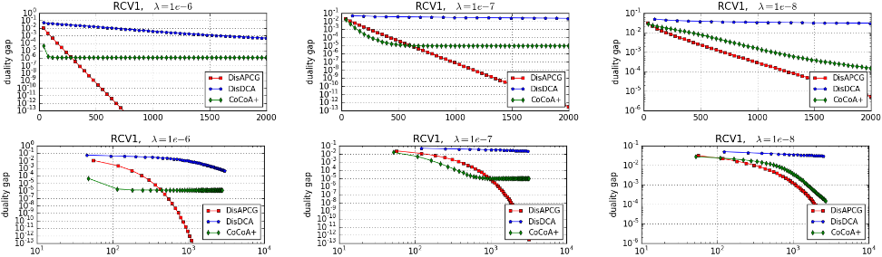
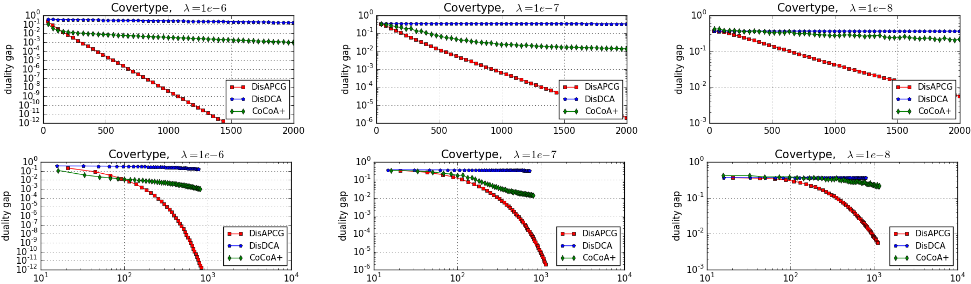
We vary λ from 10-6 to 10-8 , which is a relatively hard setting since the strong convexity parameter is small. For all settings, we use K = 16 nodes. The overall comparison is summarized in Fig.2 and Fig.3. In all settings, the CoCoA+ and our DisAPCG method outperform DisDCA a lot. For the former two, as we can see, when λ is relatively large, i.e., λ = 10-6 , the CoCoA+ solver reduces the duality gap quickly at the beginning, however, the speed slows down rapidly at an relatively accuracy level, e.g., 10-6 in the RCV1 dataset. This phenomena happens, no matter with the choice of the number of iterations for the local SDCA solver. In contrast, the DisAPCG algorithm keeps the linear convergence rate all the time and hence achieves better performance in the case that high accuracy is needed. For the most ill condition, i.e., λ = 10-8 , our DisAPCG algorithm achieve the best performance, either in terms of iterations or running time, on both datasets. It is worth mentaining that CoCoA+ is a framework that can use any local solver, not only limited in SDCA. As mentioned in Section 2.2, our algorithm can be regarded as a mini-batch version of the APCG algorithm when K = 1, which supports share-memory level parallel computing in multi-core nodes. A combination of CoCoA+ with our single-machine version of DisAPCG seems to be a good choice to further accelerate the algorithm in practice.
5 Conclusions
We have presented a distributed accelerated coordinate methods DisAPCG for the composite convex optimization problem. Our method combines the Nesterov's method and parallel structures, enjoying an accelerated convergence rate for both strongly and non-strongly convex cases. Experiments for the ERM problem show better performance camparing with several other state-of-art solvers, matching our theoretical findings as well.
Acknowledgments
The work was supported by the National Basic Research Program (973 Program) of China (No. 2013CB329403), NSFC Projects (Nos. 61620106010, 61621136008, 61332007), Tiangong Institute for Intelligent Computing, and the Youth Top-notch Talent Support Program.
@inproceedings{ijcai2017p370,
  title     = {Distributed Accelerated Proximal Coordinate Gradient Methods},
  author    = {Ren, Yong and Zhu, Jun},
  booktitle = {Proceedings of the Twenty-Sixth International Joint Conference on
               Artificial Intelligence, {IJCAI-17}},
  publisher = {International Joint Conferences on Artificial Intelligence Organization},
  editor    = {Carles Sierra},
  pages     = {2655--2661},
  year      = {2017},
  month     = {8},
  note      = {Main track},
  doi       = {10.24963/ijcai.2017/370},
  url       = {https://doi.org/10.24963/ijcai.2017/370},
}
TY - CPAPER TI - Distributed Accelerated Proximal Coordinate Gradient Methods AU - Ren, Yong AU - Zhu, Jun T2 - Proceedings of the Twenty-Sixth International Joint Conference on Artificial Intelligence, IJCAI-17 PB - International Joint Conferences on Artificial Intelligence Organization PY - 2017 SP - 2655 EP - 2661 DO - 10.24963/ijcai.2017/370 UR - https://doi.org/10.24963/ijcai.2017/370 ER -Copied
Machine-readable versions of this paper, for tools and AI agents:





