
Deep Neural Networks for High Dimension, Low Sample Size Data
Proceedings of the Twenty-Sixth International Joint Conference on Artificial Intelligence. Main track. Pages 2287-2293.
https://doi.org/10.24963/ijcai.2017/318
Keywords
- Multidisciplinary Topics and Applications: Computational Biology and e-Health
- Machine Learning: Deep Learning
- Machine Learning: Feature Selection/Construction
Abstract
Deep neural networks (DNN) have achieved breakthroughs in applications with large sample size. However, when facing high dimension, low sample size (HDLSS) data, such as the phenotype prediction problem using genetic data in bioinformatics, DNN suffers from overfitting and high-variance gradients. In this paper, we propose a DNN model tailored for the HDLSS data, named Deep Neural Pursuit (DNP). DNP selects a subset of high dimensional features for the alleviation of overfitting and takes the average over multiple dropouts to calculate gradients with low variance. As the first DNN method applied on the HDLSS data, DNP enjoys the advantages of the high nonlinearity, the robustness to high dimensionality, the capability of learning from a small number of samples, the stability in feature selection, and the end-to-end training. We demonstrate these advantages of DNP via empirical results on both synthetic and real-world biological datasets.
- [Alipanahi et al., 2015] Babak Alipanahi, Andrew Delong, Matthew T Weirauch, and Brendan J Frey. Predicting the sequence specificities of DNA-and RNA-binding proteins by deep learning. Nature Biotechnology, 2015.
- [Amaldi and Kann, 1998] Edoardo Amaldi and Viggo Kann. On the approximability of minimizing nonzero variables or unsatis- fied relations in linear systems. Theoretical Computer Science, 209(1):237-260, 1998.
- [Bach, 2014] Francis Bach. Breaking the curse of dimensionality with convex neural networks. arXiv:1412.8690, 2014.
- [Bahdanau et al., 2014] Dzmitry Bahdanau, Kyunghyun Cho, and Yoshua Bengio. Neural machine translation by jointly learning to align and translate. arXiv:1409.0473, 2014.
- [Bengio et al., 2005] Yoshua Bengio, Nicolas L Roux, Pascal Vin- cent, Olivier Delalleau, and Patrice Marcotte. Convex neural net- works. In Advances in Neural Information Processing Systems, pages 123-130, 2005.
- [Breiman, 2001] Leo Breiman. Random forests. Machine Learn- ing, 45(1):5-32, 2001.
- [Consortium, 2015] 1000 Genomes Project Consortium. A global reference for human genetic variation. Nature, 526(7571):68-74, 2015.
- [Duchi et al., 2011] John Duchi, Elad Hazan, and Yoram Singer. Adaptive subgradient methods for online learning and stochastic optimization. Journal of Machine Learning Research, 12:2121- 2159, 2011.
- [Evgeniou and Pontil, 2007] A Evgeniou and Massimiliano Pontil. Multi-task feature learning. Advances in Neural Information Pro- cessing Systems, 19:41, 2007.
- [Fan and Li, 2006] Jianqing Fan and Runze Li. Statistical chal- lenges with high dimensionality: feature selection in knowledge discovery. arXiv:math/0602133, 2006.
- [Friedman et al., 2000] Jerome Friedman, Trevor Hastie, and Robert Tibshirani. The Elements of Statistical Learning. first edition, 2000.
- [Friedman, 2001] Jerome Friedman. Greedy function approxima- tion: a gradient boosting machine. Annals of Statistics, pages 1189-1232, 2001.
- [Glorot and Bengio, 2010] Xavier Glorot and Yoshua Bengio. Un- derstanding the difficulty of training deep feedforward neural net- works. In Proceedings of International Conference on Artificial Intelligence and Statistics, pages 249-256, 2010.
- [Glorot et al., 2011] Xavier Glorot, Antoine Bordes, and Yoshua Bengio. Deep sparse rectifier neural networks. In Proceedings of International Conference on Artificial Intelligence and Statis- tics, pages 315-323, 2011.
- [Guyon and Elisseeff, 2003] Isabelle Guyon and André Elisseeff. An introduction to variable and feature selection. Journal of Ma- chine Learning Research, 3:1157-1182, 2003.
- [He et al., 2015] Kaiming He, Xiangyu Zhang, Shaoqing Ren, and Jian Sun. Deep residual learning for image recognition. arXiv:1512.03385, 2015.
- [Hinton et al., 2012] Geoffrey Hinton, Li Deng, Dong Yu, George E Dahl, Abdel-rahman Mohamed, Navdeep Jaitly, Andrew Senior, Vincent Vanhoucke, Patrick Nguyen, Tara N Sainath, and Brian Kingsbury. Deep neural networks for acoustic modeling in speech recognition: the shared views of four research groups. IEEE Signal Processing Magazine, 29(6):82-97, 2012.
- [Kalousis et al., 2007] Alexandros Kalousis, Julien Prados, and Melanie Hilario. Stability of feature selection algorithms: a study on high-dimensional spaces. Knowledge and Information Sys- tems, 12(1):95-116, 2007.
- [Leung et al., 2016] Michael KK Leung, Andrew Delong, Babak Alipanahi, and Brendan J Frey. Machine learning in genomic medicine: a review of computational problems and data sets. Pro- ceedings of the IEEE, 104(1):176-197, Jan 2016.
- [Li et al., 2005] Fan Li, Yiming Yang, and Eric P Xing. From lasso regression to feature vector machine. In Advances in Neural In- formation Processing Systems, pages 779-786, 2005.
- [Li et al., 2015] Yifeng Li, Chih-Yu Chen, and Wyeth W Wasser- man. Deep feature selection: Theory and application to iden- tify enhancers and promoters. In International Conference on Research in Computational Molecular Biology, pages 205-217. Springer, 2015.
- [Pati et al., 1993] Yagyensh Chandra Pati, Ramin Rezaiifar, and PS Krishnaprasad. Orthogonal matching pursuit: recursive func- tion approximation with applications to wavelet decomposition. In Proceedings of 27th Asilomar Conference on Signals, Systems and Computers, pages 40-44, 1993.
- [Perkins et al., 2003] Simon Perkins, Kevin Lacker, and James Theiler. Grafting: Fast, incremental feature selection by gradi- ent descent in function space. Journal of Machine Learning Re- search, 3:1333-1356, 2003.
- [Ravikumar et al., 2007] Pradeep Ravikumar, Han Liu, John Laf- ferty, and Larry Wasserman. Spam: Sparse additive models. In Advances in Neural Information Processing Systems, 2007.
- [Srivastava et al., 2014] Nitish Srivastava, Geoffrey E Hinton, Alex Krizhevsky, Ilya Sutskever, and Ruslan Salakhutdinov. Dropout: a simple way to prevent neural networks from overfitting. Journal of Machine Learning Research, 15(1):1929-1958, 2014.
- [Tewari et al., 2011] Ambuj Tewari, Pradeep K Ravikumar, and In- derjit S Dhillon. Greedy algorithms for structurally constrained high dimensional problems. In Advances in Neural Information Processing Systems, pages 882-890, 2011.
- [Tibshirani, 1996] Robert Tibshirani. Regression shrinkage and se- lection via the lasso. Journal of the Royal Statistical Society. Series B (Methodological), pages 267-288, 1996.
- [Xiong et al., 2015] Hui Y Xiong, Babak Alipanahi, Leo J Lee, Hannes Bretschneider, Daniele Merico, Ryan KC Yuen, Yimin Hua, Serge Gueroussov, Hamed S Najafabadi, Timothy R Hughes, et al. The human splicing code reveals new in- sights into the genetic determinants of disease. Science, 347(6218):1254806, 2015.
- [Xu et al., 2014] Zhixiang Xu, Gao Huang, Kilian Q Weinberger, and Alice X Zheng. Gradient boosted feature selection. In Pro- ceedings of the 20th ACM SIGKDD International Conference on Knowledge Discovery and Data Mining, pages 522-531. ACM, 2014.
- [Yamada et al., 2014] Makoto Yamada, Wittawat Jitkrittum, Leonid Sigal, Eric P Xing, and Masashi Sugiyama. High- dimensional feature selection by feature-wise kernelized lasso. Neural Computation, 26(1):185-207, 2014.
- [Yamada et al., 2016] Makoto Yamada, Jiliang Tang, Jose Lugo- Martinez, Ermin Hodzic, Raunak Shrestha, Avishek Saha, Hua Ouyang, Dawei Yin, Hiroshi Mamitsuka, Cenk Sahinalp, Pre- drag Radivojac, Filippo Menczer, and Yi Chang. Ultra high- dimensional nonlinear feature selection for big biological data. arXiv:1608.04048, 2016.
References were extracted automatically from the PDF and may contain errors.
Full text extracted automatically from the PDF; figures, tables and equations may differ. The PDF is the version of record.
1 Introduction
In bioinformatics, phenotype prediction using genetic variants suffers from the growing challenges of high dimensionality and low sample size. Until 2008, biologists had identified 15 million genetic variants (single-nucleotide polymorphisms or SNP) for Homo Sapiens. The number of recognized genetic variants quadrupled in 2011 and increased to 150 million in 2016. In contrast, only thousands of samples are available [Consortium, 2015]. This kind of high dimension, low sample size (HDLSS) data is also vital for scientific discoveries in other areas such as chemistry, financial engineering, and etc [Fan and Li, 2006]. When processing this kind of data, the severe overfitting and high-variance gradients are the major challenges for the majority of machine learning algorithms [Friedman et al., 2000].
Feature selection has been widely regarded as one of the most powerful tools to analyze the HDLSS data. Firstly, selecting the optimal subset of features reduces the size of feature space, thereby alleviating the risk of overfitting. Secondly, new scientific knowledge can be discovered through selecting features. For instance, selecting features from genotype-cancer datasets helps accumulate the knowledge of cancer-related genetic variants. However, selecting the optimal subset of features is known to be NPhard [Amaldi and Kann, 1998]. Instead, a large body of compromised methods for feature selection have been proposed. Amongst them, a line of representative methods includes Lasso [Tibshirani, 1996] pursue sparse linear models. Unfortunately, sparse linear models ignore the nonlinear input-output relations and interactions among features, both of which have been proved to be important in explaining the missing heritability in phenotype prediction. Although some attempts have been made to achieve nonlinear feature selection via kernel methods [Li et al., 2005; Yamada et al., 2014] or gradient boosted tree [Xu et al., 2014], almost all of them address the curse of dimensionality under the blessing of large sample size.
The deep neural networks (DNN) methods light up new scientific discoveries, in particular, to understand biological processes from genotype to phenotype. Firstly, DNN has achieved breakthroughs in modeling nonlinearity in wide applications, such as image recognition [He et al., 2015], machine translation [Bahdanau et al., 2014], and speech recognition [Hinton et al., 2012]. The deeper architecture of a DNN is, the more complex relations it can model. Therefore, DNN is qualified to model mutual interactions among DNA, RNA, and proteins which are even more complex than those aforementioned applications [Leung et al., 2016]. Secondly, the central dogma of biology states that the genotype decides the phenotype by following a hierarchical path, i.e., from DNA to RNA and further to protein. DNN is born to mimic such multi-layer biological processes. Moreover, DNN has harvested initial successes in bioinformatics for modeling splicing [Xiong et al., 2015] and sequence specificity [Alipanahi et al., 2015].
In the aforementioned applications, large sample size greatly contributes to the state-of-the-art performance of DNN. Nevertheless, few efforts have been devoted to applying DNN to the HDLSS problem. Estimating a huge amount of parameters for DNN using abundant samples may suffer from severe overfitting, not to mention the HDLSS setting.
To address the challenges of the HDLSS data, we propose an end-to-end DNN model called Deep Neural Pursuit (DNP). DNP simultaneously selects features and learns a classifier to alleviate severe overfitting caused by high dimensionality. By averaging over multiple dropouts, DNP is robust and stable to high-variance gradients resulting from the small sample size. From the perspective of feature selection, the DNP model selects features greedily and incrementally, similar to the matching pursuit [Pati et al., 1993]. More concretely, starting from an empty subset of features and a bias, the proposed DNP method incrementally selects an individual feature according to the backpropagated gradients. Meantime, once more features are selected, DNP is updated using the backpropagation algorithm.
The main contribution of this paper is to tailor the DNN for the HDLSS setting using feature selection and multiple dropouts. On the synthetic and real-world HDLSS datasets, the proposed DNP performs comparably or significantly better than sparse linear models and kernel-based/gradientboosted-tree-based nonlinear feature selection methods.
2 RelatedWork
In this section, we discuss feature selection methods that are used to analyze the HDLSS data including linear, nonlinear and incremental methods.
Learning the linear model with sparsity-inducing regularizer is one of the dominating feature selection methods for the HDLSS data. For instance, Lasso [Tibshirani, 1996] minimizes the objective function penalized by the l1 norm of feature weights, leading to a sparse model. Unfortunately, Lasso considers only the linear input-output dependency but ignores the nonlinearity and interactions among features.
Kernel methods are often used for nonlinear feature selection. Feature Vector Machine (FVM) [Li et al., 2005] nonlinearly transforms each feature and label using the kernel function and it learns a sparse model using the new features and labels to achieve nonlinear feature selection. HSIC-Lasso [Yamada et al., 2014] improves FVM by allowing different kernel functions for features and labels. HSIC-Lasso also selects less redundant features. LAND [Yamada et al., 2016] further accelerates HSIC-Lasso for data with large sample size via kernel approximation and distributed computation.
Decision tree models are also qualified for modeling nonlinear input-output relations. As an ensemble of decision trees, random forests [Breiman, 2001] select a feature according to its contribution to the model. One of the selection criteria is to measure how much the performance decreases by permuting the specific feature. Gradient boosted feature selection (GBFS) [Xu et al., 2014] penalizes the usage of features that are not yet used during the construction of each tree. By early stopping of boosting, GBFS obtains an ensemble of tree models with only a subset of features incorporated.
Unfortunately, the aforementioned nonlinear methods, including FVM, random forests and GBFS, require training data with large sample size. HSIC-Lasso and LAND fits the HDLSS setting. However, compared to the proposed DNP model which is end-to-end, HSIC-Lasso and LAND are twostage algorithms which separate feature selection from the classification.
Besides DNP method, there exist other greedy and incremental feature selection algorithms. For example, SpAM [Ravikumar et al., 2007] sequentially selects an individual
�� � � ��
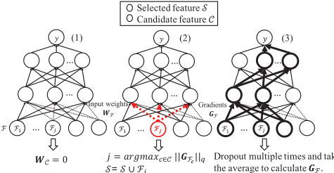
Figure 1: (1) The selected features and the corresponding subnetwork. (2) The selection of a single feature. (3) Calculate gradients with lower variance via multiple dropouts.
feature in an additive manner, thereby missing important interactions among features. For multilayer perceptron with one hidden layer, Grafting method [Perkins et al., 2003] incrementally adds connections or hidden neurons based on gradient-related heuristics. Similarly, convex neural network [Bengio et al., 2005] dynamically adds hidden neurons which maximize the correlation with negative gradients of the objective function. For one thing, Grafting and convex neural network only consider single hidden layer. For another, Grafting and convex neural network differ from DNP in the motivation. DNP aims at learning from the HDLSS data. In contrast, Grafting focuses on the acceleration of algorithms and convex neural network focuses on the theoretical understanding of neural networks.
Deep feature selection (DFS) [Li et al., 2015], which selects features in the context of DNN, shares a similar motivation to DNP. DFS learns sparse one-to-one connections between input features and neurons in the first hidden layer. However, according to our experiments, DFS fails to achieve sparse connections when facing the HDLSS data.
3 The DNPModel
We first introduce notations throughout this paper. F ∈ Rd denotes the input feature space in the d-dimension. X = (x1, x2, . . . , xn) and y = (y1, y2, . . . , yn)T denote the data matrix of n samples and their corresponding labels, respectively. In the HDLSS setting, d ≫ n. Moreover, f(X|W) stands for a feed-forward neural network whose weights of all connections are denoted by W and G stands for the back propagated gradients for W. Particularly, WF denotes the input weights, which are the weights of connections between the input layer and the first hidden layer, andGF indicates the corresponding gradients. We consider a multilayer perceptron with Rectifier Linear Units (ReLU) [Glorot et al., 2011]. An illustration of the neural network is shown in Fig. 1.
Under the HDLSS setting, we face the risk of overfitting and the challenge of high-variance gradients. In the following sections, we first detail the DNP model for feature selection which alleviates overfitting caused by the high dimensionality. And we present the use of multiple dropouts to handle high-variance gradients caused by the small sample size. Then, we discuss the stagewise and stepwise DNP. Finally, we analyze the time complexity of DNP.
3.1 DNP for High Dimensionality
For a feed-forward neural network, we select a specific input feature if at least one of the connections associated with that feature has non-zero weight. To achieve this goal, we place the lp,1 norm to constrain the input weights, i.e., ‖WF‖p,1. We use WFj to denote the weights associated with the j-th input node inWF. We can define the lp,1 norm of the input weights as ‖WF‖p,1 = ∑j ‖WFj ‖p, where ‖ · ‖p is the lp norm on a vector. One effect of the lp,1 norm is to enforce the group sparsity [Evgeniou and Pontil, 2007] and here we assume that weights inWFj form a group. A general form of the objective function for training the feed-forward network in formulated as:
Without loss of generality, we only consider the binary classification problem and use the logistic loss in problem (1). Extensions to multi-class classification, regression or unsupervised reconstruction are very easy.
To directly optimize problem (1) over the HDLSS data is highly tricky for two reasons. Firstly, directly minimizing the lp,1-constrained problem is difficult for the back propagation algorithm [Bach, 2014]. Secondly, direct optimization using all features easily gets stuck in a local optimum which suffers from severe overfitting. For instance, we may achieve meaningless zero training loss on the HDLSS data. Instead, we optimize problem (1) in a greedy and incremental manner.
The main idea of the proposed DNP is that initially, based on a limited amount of samples, we optimize problem (1) over a small sub-network containing a small subset of features, which is less difficult. We show this small sub-network with solid circles and lines in Fig. 1(1). Then, the information obtained during the training process, in turn, guides us to incorporate more features, and the sub-network serves as the initialization for a larger sub-network with more features involved.
The DNP method enjoys two advantages. First of all, the optimization improves to a large extent. DNP trains far smaller sub-networks at early stages and can find better local optima by using previous sub-networks as the initialization. Secondly, DNP simultaneously selects features and minimizes the training loss over the labeled data in an end-to-end manner, thereby outperforming some feature selection methods whose selection process is independent of the learning process [Guyon and Elisseeff, 2003].
The whole process of the feature selection in the DNP is introduced as follows. We graphically illustrate DNP's greedy feature selection in Fig. 1 and detail the learning process in Algorithm 1. We maintain two sets, i.e., a selected set S and a candidate set C, with S ∪ C = F.
Initially, S starts from a bias to avoid the case that all ReLU hidden units are inactive. Except the weights corresponding to the bias, all weights in the neural network are initialized to be zero. Upon the selected set S, input weightsWF comprise of selected input weights WS, which are input weights associated with features in S, and candidate weights WC. We update the whole neural network until convergence while fixing
Algorithm 1 Deep Neural Pursuit
- 1: Input: X ∈ Rn×d , y ∈ Rn , the maximum number of selected features k.
- 2: Initialize: S = {bias}, C = F andWC = 0.
- 3: while |S| ≤ k + 1 do
- 4: Fix candidate weightsWC = 0;
- 5: Update weights of hidden layer and inputWS;
- 6: Dropout multiple times and average out GFc ;
- 7: j = argmaxc∈C ‖GFc ‖q;
- 8: Update learning rates using Adagrad;
- 9: InitializeWFj with Xavier Initializer;
- 10: S = S ∪Fj and C = C \ Fj;
11: end while
all candidate weights WC to zero (i.e., steps 4 and 5 of Algorithm 1). In Fig. 1(1), we plot S and C with solid circles and dotted circles, respectively. All dotted connections are fixed zero. Then, GF is employed to select one feature, say the jth one from C (step 7). After that, WF is updated by initializing newly selected input weights WFj with Xavier Initializer [Glorot and Bengio, 2010] and reusing earlier weights WS (step 9). S and C are updated by adding and removing j, respectively (step 10).
One question is how to select features using GF. Without loss of generality, we assume that all features are normalized. In this case, the gradient's magnitude implies howmuch the objective function may decrease by updating the corresponding weight [Perkins et al., 2003]. Similarly, the norm of a group of gradients infers how much the loss may decrease by updating this group of weights together. According to [Tewari et al., 2011], there exists an equivalence between minimizing the lp,1 norm in problem (1) and greedily selecting features with the maximum lq norm of gradients, where q satisfies 1/p + 1/q = 1. Thus, we assume that the larger the ‖GFj ‖q is, the more jth feature contributes to minimizing problem (1). Consequently, we select the feature with the maximum ‖GFj ‖q. Throughout our experiments, we choose p = q = 2 provided that our empirical comparisons among different settings of p show a limited difference. On the other hand, DNP can satisfy the norm constraint, i.e., ||WF||p,1 ≤ λ, by early stopping at the kth iteration. We illustrate the selection of a single feature in Fig. 1(2).
3.2 DNP for Small Sample Size
Due to the small sample size, the backpropagated gradients in DNP are especially of high variance, making selecting features according to gradients misleading. As shown in Fig. 1(3), DNP utilizes multiple dropouts technique to avoid highvariance gradients. As a regularizer, dropout [Srivastava et al., 2014] randomly drops neurons and features during forward training and back propagation. Therefore gradients G are calculated on the sub-network composed of the rest neurons.
Multiple dropouts could improve our DNP method in the following two algorithmic aspects. Firstly, according to step 6 of Algorithm 1, DNP randomly drops neurons multiple times, computes GFc based on the remaining neurons and connections, and averages multiple GFc . Such multiple dropouts technique obtains averaged gradients with low variance.
Secondly and more importantly, multiple dropouts empower DNP with the stable feature selection. Stability, as a vital criterion for feature selection, indicates that identical features should be consistently selected even using slightly changed training datasets [Kalousis et al., 2007]. Multiple dropouts combine selected features over many random subnetworks to make the DNP method more stable and powerful.
3.3 Stagewise vs Stepwise
Updating input weights WS in step 5 of Algorithm 1 has two choices, i.e., the stagewise and stepwise approaches. Before proceeding to introduce the two choices, we first split WS into two parts. The first part isWFj which contains input weights connecting to the jth input node for the newly selected feature Fj, and the other part is WS\Fj . The stagewise approach updates WFj only in current iteration, while keeping WS\Fj unchanged. The gradient boosting method [Friedman, 2001] is a representative stagewise method. Different from the stagewise approach, the stepwise approach updates selected weights WS altogether. One representative method named Orthogonal Matching Pursuit (OMP) [Pati et al., 1993] minimizes the objective function every time a new feature is added.
Both of the boosting and OMP methods inspire our DNP method. Instead of directly using pure stagewise or pure stepwise updating, we combine both approaches. In detail, we dynamically adapt the learning rate for each weight according to the Adagrad [Duchi et al., 2011]. For each weight in the neural network, its learning rate decreases with the sum of gradients in all the past iterations. As a result, like the stepwise approach, all selected weights WS enjoy updates but, like the stagewise approach, newly selected features WFj enjoy more.
3.4 Time Complexity
The time complexity of DNP is dominated by the backpropagation which is O(hknd), where h is a constant decided by the network structure of DNP. Thus, the time complexity grows linearly with respect to the number of selected features k, the sample size n, and the feature dimension d. In comparison, the complexity of HSIC-Lasso grows cubicly with respect to the sample size, i.e., O(kn3d) [Yamada et al., 2016].
4 Experiments
In this section, we empirically evaluate the performance of the proposed DNP model.
We compare the proposed DNP method with three representative feature selection algorithms, including l1-penalized logistic regression (LogR-l1), gradient boosted feature selection (GBFS) [Xu et al., 2014], and HSIC-Lasso [Yamada et al., 2014]. LogR-l1 performs linear feature selection with the l1 regularization for classification problems. GBFS 1 is a representative of nonlinear feature selection based on gradient boosted tree. GBFS penalizes the usage of features that are not yet used when constructing each tree and by early stopping, it learns an ensemble of regression trees with only a subset of features involved. HSIC-Lasso 2 is also nonlinear but based on kernels, in which it learns a sparse model on kernelized labels and features. HSIC-Lasso is also recognized as the state-of-the-art minimum redundancy maximum relevance (mRMR) based methods. However, it cannot select features and learn a classifier simultaneously. Thus, we adapt it by utilizing SVM with the RBF kernel as the classifier after feature selection.
1 GBFS code: http://www.cse.wustl.edu/˜xuzx/ research/code/GBFS.zip
4.1 Experiments on Synthetic Data
The proposed DNP method has two goals. The first is to identify features that the labels truly depend on, which is measured by the F1 score of correct selection of true features. The second is to learn an accurate classifier based on selected features, which is evaluated by the test AUC score. We first synthesize highly complex and nonlinear data to investigate the performance of different algorithms towards the two goals.
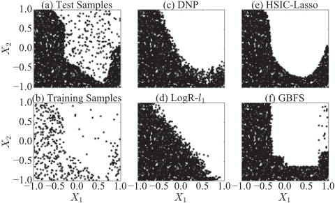
To generate the synthetic data, we firstly draw input samples X from the uniform distribution U(-1, 1), where the feature dimension d is fixed to be 10,000. Afterwards, we obtain the corresponding labels by passing X into the feedforward neural network with {50, 30, 15, 10} ReLU hidden units in four hidden layers. Such knowledge of the network structure generating the synthetic data is unknown to DNP. Input weights connecting with the first m dimensions, i.e. WF1...m , are randomly sampled from a Gaussian distribution N(0, 0.5). The remaining connections are kept zero. Thus, F1...m serve as the true features that decide the label. In order to add noises into data, we randomly flip 5% labels. For each setting of m, we generate 800 training samples, 200 validation samples, and 7,500 test samples, hence the sample sizes of the training and validation sets are far smaller than the dimensionality d.
When m = 2, we visualize the decision boundaries learned by different algorithms in Fig. 2. As expected, LogR-l1 only learns a linear decision boundary which is insufficient for highly complex and nonlinear data. The GBFS uses the regression tree as a base learner, thereby achieving an axisparallel decision boundary. The HSIC-Lasso and the proposed DNP not only model the nonlinear decision boundaries but also exactly identify the two true features. As Table 1 shows, the F1 scores of feature selection reach 1 for both methods.
2 HSIC-Lasso code: http://www.makotoyamada-ml. com/software.html
We further compare the performance of different algorithms as shown in Table 1. The test AUC scores and F1 scores are averaged across five random generated datasets. In terms of the test AUC score, DNP and HSIC-Lasso both show superior performance over others. DNP performs best on all the datasets and significantly outperforms HSIC-Lasso when m = 10 in terms of the t-test (p-value < 0.05). LogR-l1 is significantly outperformed by DNP on three out of four synthetic datasets and tends to be comparable when m = 25. In terms of the F1 score for feature selection, DNP performs the best on all datasets and it even outperforms the most competitive baseline, HSIC-Lasso, by 8.65% on average. GBFS consistently performs worst in terms of both classification and feature selection.
4.2 Experiments on Real-World Biological Datasets
To investigate the performance of DNP on the real-world datasets, we use six public biological datasets 3 , all of which suffer from the HDLSS problem. The statistics of these datasets are shown in Table 2. We report the average results for 10 times random split with 80% data for training, 10% for validation, and 10% for testing.
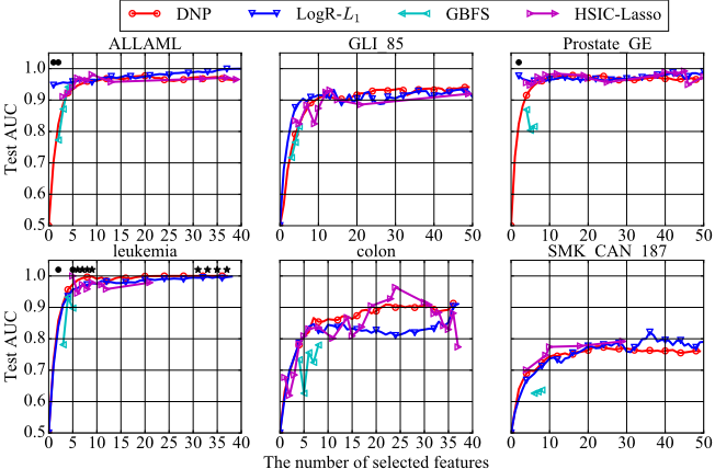
In Fig. 3, we investigate the average test AUC scores with respect to the number of selected features. DNP selects a single feature in each iteration. As a result, in Fig. 3, the performance curve of DNP is equivalent to how the test AUC scores change with respect to the number of iterations. On all six datasets, test AUC scores of DNP converge quickly within fewer than 10 iterations. For LogR-l1, GBFS, and HSICLasso, the number of selected features is tuned by choosing the appropriate hyper-parameters. We use a circle as an indicator when DNP is outperformed by the best baseline and a star when DNP outperforms the best baseline significantly (t-test, p-value < 0.05).
3 Biological datasets: http://featureselection.asu. edu/datasets.php
| True Dim | 2 | 5 | 10 | 25 | |
|---|---|---|---|---|---|
| LogR-l1 | AUC | 0.868 | 0.826 | 0.755 | 0.661 |
| Std | 0.003 | 0.001 | 0.014 | 0.017 | |
| GBFS | AUC | 0.748 | 0.721 | 0.757 | 0.565 |
| Std | 0.184 | 0.130 | 0.011 | 0.029 | |
| HSIC-Lasso | AUC | 0.948 | 0.881 | 0.747 | 0.642 |
| Std | 0.003 | 0.001 | 0.003 | 0.007 | |
| DNP | AUC | 0.926 | 0.887 | 0.813 | 0.650 |
| Std | 0.005 | 0.023 | 0.025 | 0.016 | |
| LogR-l1 F1 score | 0.141 | 0.313 | 0.364 | 0.266 | |
| Std | 0.025 | 0.045 | 0.046 | 0.035 | |
| GBFS | F1 score | 0.182 | 0.050 | 0.429 | 0.105 |
| Std | 0.183 | 0.056 | 0.048 | 0.052 | |
| HSIC-Lasso | F1 score | 1.000 | 0.889 | 0.667 | 0.253 |
| Std | 0.000 | 0.000 | 0.000 | 0.033 | |
| DNP | F1 score | 1.000 | 0.862 | 0.857 | 0.378 |
| Std | 0.000 | 0.075 | 0.085 | 0.054 |
| Data | Colon | Prostate GE | Leukemia |
|---|---|---|---|
| Sample size | 62 | 102 | 72 |
| Dimensionality | 2,000 | 5,966 | 7,070 |
| Data | ALLAML | SMK CAN 87 | GLI 85 |
| Sample size | 72 | 187 | 85 |
| Dimensionality | 7,129 | 19,993 | 22,283 |
On the leukemia dataset, the proposed DNP method significantly outperforms the best baseline no matter how many features are selected. For the ALLAML and Prostate GE dataset, LogR-l1 serves as a competitive baseline as it outperforms other methods when few features are selected. However, DNP achieves a comparable test AUC score when more features are involved. For the other three datasets, DNP outperforms GBFS significantly and performs comparable to LogR-l1 and HSIC-Lasso. On average across six real-world datasets, DNP outperforms the most competitive baseline, HSIC-Lasso, by 2.53% in terms of the average test AUC score. In summary, DNP can achieve comparable or improved performance over baselines on the six real-world datasets.
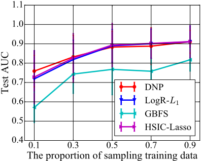
To investigate the effect of the size of the training data, we compare DNP with the baselines by varying the sample size for training, while the sample sizes for validation and test are kept fixed. Fig. 4 shows the average test AUC scores across six real-world datasets. All the methods in comparison suffer as the training sample size decreases. GBFS, designed for large sample size, suffers the most. LogR-l1, HSIC-Lasso, and DNP perform similarly in small sample size. However, when only 10% or 30% training samples are used, DNP slightly outperforms other baselines.
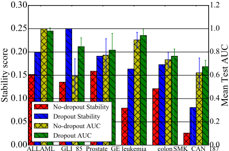
To see the role of multiple dropouts, we compare the performance of DNP with and without multiple dropouts in Fig. 5. According to the results, we can see that multiple dropouts can improve the test AUC score on five out of six datasets.
We measure the stability of the algorithms with the Tanimoto distance [Kalousis et al., 2007]. In detail, on a pair of training sets, DNP selects feature subsets S1 and S2, respectively. Then the Tanimoto distance measures the similarity between S1 and S2 as Similarity(S1, S2) = 1 - |S1|+|S2|-2|S1∩S2| |S1|+|S2|-|S1∩S2| , where | · | represents the cardinality for a set. Then, we measure the stability of DNP by averaging the similarities calculated from all pairs of training sets generated from 10-fold cross validation. A higher stability score implies a more stable algorithm. As shown in Fig. 5, DNP with multiple dropouts is clearly more stable than DNP without dropout on the all six datasets.
| Data | Colon | Prostate GE | Leukemia |
|---|---|---|---|
| DNP's best depth | 2 | 4 | 3 |
| Data | ALLAML | SMK CAN 87 | GLI 85 |
| DNP's best depth | 3 | 4 | 3 |
Finally, we investigate how the hyper-parameters influence the performance of DNP. We vary the number of hidden layers from one to five. For DNP model with the specific number of hidden layers, we calculate the average test AUC score of 10 times random split. In Table 3, we list the number of hidden layers leading to the best test AUC score. On five realworld datasets, DNP with three or four hidden layers outperforms that with one, two or five hidden layers. The results coincide with our motivation that deeper neural networks are more qualified for complex datasets. Meantime, due to the small sample size, training DNNs with more hidden layers is extremely challenging, which incurs inferior performances.
5 Conclusions
In this paper, we propose a DNP model tailored for the high dimension, low sample size data. DNP can select features in a nonlinear way. With an incremental manner to select features, DNP is robust to high dimensionality. By using the multiple dropouts technique, DNP can learn from a small number of samples and is stable for feature selection. Moreover, the training of DNP is end-to-end. Empirical results verify its good performance in both classification and feature selection.
In the future, we plan to use sophisticated network architectures in replace of a simple multi-layer perceptron and apply DNP to more domains that suffer from the HDLSS problem.
Acknowledgements
We thank the support of National Grant Fundamental Research (973 Program) of China under Project 2014CB340304 and Hong Kong CERG projects 16211214, 16209715 and 16244616. Yu Zhang is supported by National Natural Science Foundation of China under Projects 61473087 and 61673202 and Natural Science Foundation of Jiangsu Province under Project BK20141340.
@inproceedings{ijcai2017p318,
  title     = {Deep Neural Networks for High Dimension, Low Sample Size Data},
  author    = {Liu, Bo and Wei, Ying and Zhang, Yu and Yang, Qiang},
  booktitle = {Proceedings of the Twenty-Sixth International Joint Conference on
               Artificial Intelligence, {IJCAI-17}},
  publisher = {International Joint Conferences on Artificial Intelligence Organization},
  editor    = {Carles Sierra},
  pages     = {2287--2293},
  year      = {2017},
  month     = {8},
  note      = {Main track},
  doi       = {10.24963/ijcai.2017/318},
  url       = {https://doi.org/10.24963/ijcai.2017/318},
}
TY - CPAPER TI - Deep Neural Networks for High Dimension, Low Sample Size Data AU - Liu, Bo AU - Wei, Ying AU - Zhang, Yu AU - Yang, Qiang T2 - Proceedings of the Twenty-Sixth International Joint Conference on Artificial Intelligence, IJCAI-17 PB - International Joint Conferences on Artificial Intelligence Organization PY - 2017 SP - 2287 EP - 2293 DO - 10.24963/ijcai.2017/318 UR - https://doi.org/10.24963/ijcai.2017/318 ER -Copied
Machine-readable versions of this paper, for tools and AI agents:





