
Regional Concept Drift Detection and Density Synchronized Drift Adaptation
Proceedings of the Twenty-Sixth International Joint Conference on Artificial Intelligence. Main track. Pages 2280-2286.
https://doi.org/10.24963/ijcai.2017/317
Keywords
- Machine Learning: Time-series/Data Streams
- Machine Learning: Online Learning
- Machine Learning: Classification
Abstract
In data stream mining, the emergence of new patterns or a pattern ceasing to exist is called concept drift. Concept drift makes the learning process complicated because of the inconsistency between existing data and upcoming data. Since concept drift was first proposed, numerous articles have been published to address this issue in terms of distribution analysis. However, most distribution-based drift detection methods assume that a drift happens at an exact time point, and the data arrived before that time point is considered not important. Thus, if a drift only occurs in a small region of the entire feature space, the other non-drifted regions may also be suspended, thereby reducing the learning efficiency of models. To retrieve non-drifted information from suspended historical data, we propose a local drift degree (LDD) measurement that can continuously monitor regional density changes. Instead of suspending all historical data after a drift, we synchronize the regional density discrepancies according to LDD. Experimental evaluations on three public data sets show that our concept drift adaptation algorithm improves accuracy compared to other methods.
- [Bifet and Gavaldà, 2009] Albert Bifet and Ricard Gavaldà, "Adaptive learning from evolving data streams," in Proceedings of the Eighth International Symposium on Intelligent Data Analysis, pp. 249-260: Springer, 2009.
- [Bifet, et al., 2010] Albert Bifet, Geoff Holmes, Richard Kirkby, and Bernhard Pfahringer, "MOA: Massive online analysis," The Journal of Machine Learning Research, vol. 99, pp. 1601-1604, 2010.
- [Brzeziński and Stefanowski, 2011] Dariusz Brzeziński and Jerzy Stefanowski, "Accuracy updated ensemble for data streams with concept drift," in International Conference on Hybrid Artificial Intelligence Systems, pp. 155-163: Springer, 2011.
- [Elwell and Polikar, 2011] Ryan Elwell and Robi Polikar, "Incremental learning of concept drift in nonstationary environments," (in eng), IEEE Transactions on Neural Networks, Research Support, U.S. Gov't, Non-P.H.S. vol. 22, no. 10, pp. 1517-31, Oct 2011.
- [Frias-Blanco, et al., 2015] Isvani Frias-Blanco, Jose del Campo-Avila, Gonzalo Ramos-Jimenes, Rafael Morales- Bueno, Agustin Ortiz-Diaz, and Yaile Caballero-Mota, "Online and Non-Parametric Drift Detection Methods Based on Hoeffding's Bounds," IEEE Transactions on Knowledge and Data Engineering, vol. 27, no. 3, pp. 810- 823, 2015.
- [Gama and Castillo, 2006] João Gama and Gladys Castillo, "Learning with local drift detection," in International Conference on Advanced Data Mining and Applications, pp. 42-55: Springer, 2006.
- [Gama, et al., 2014] João Gama, Indrė Zliobaitė, Albert Bifet, Mykola Pechenizkiy, and Abdelhamid Bouchachia, "A survey on concept drift adaptation," ACM Computing Surveys, vol. 46, no. 4, pp. 1-37, 2014.
- [Harel, et al., 2014] Maayan Harel, Shie Mannor, Ran El- Yaniv, and Koby Crammer, "Concept drift detection through resampling," in Proceedings of the Thirty-first International Conference on Machine Learning, pp. 1009-1017, 2014.
- [Ikonomovska and Gama, 2008] Elena Ikonomovska and Joao Gama, "Learning Model Trees from Data Streams," in Proceedings of the Eleventh International Conference on Discovery Science, pp. 52-63, Berlin: Springer, 2008.
- [Ikonomovska, et al., 2011] Elena Ikonomovska, João Gama, and Sašo Džeroski, "Learning model trees from evolving data streams," Data Mining and Knowledge Discovery, vol. 23, no. 1, pp. 128-168, 2011.
- [Ikonomovska, et al., 2009] Elena Ikonomovska, João Gama, Raquel Sebastião, and Dejan Gjorgjevik, "Regression Trees from Data Streams with Drift Detection," in Proceedings of the Twelfth International Conference on Discovery Science, pp. 121-135, Berlin: Springer, 2009.
- [Katakis, et al., 2009] Ioannis Katakis, Grigorios Tsoumakas, Evangelos Banos, Nick Bassiliades, and Ioannis Vlahavas, "An adaptive personalized news dissemination system," Journal of Intelligent Information Systems, vol. 32, no. 2, pp. 191-212, 2009.
- [Li, et al., 2016] Peipei Li, Lu He, Xuegang Hu, Yuhong Zhang, Lei Li, and Xindong Wu, "Concept based short text stream classification with topic drifting detection," in Proceedings of the Sixteenth International Conference on Data Mining, pp. 1009-1014, 2016.
- [Liu, et al., 2017] Anjin Liu, Guangquan Zhang, and Jie Lu, "Fuzzy time windowing for gradual concept drift adaptation," in Proceedings of the Twenty-sixth IEEE International Conference on Fuzzy Systems, Naples Italy: IEEE, 2017.
- [Losing, et al., 2016] Viktor Losing, Barbara Hammer, and Heiko Wersing, "KNN Classifier with Self Adjusting Memory for Heterogeneous Concept Drift," in Proceedings of the Sixteenth IEEE International Conference on Data Mining, 2016.
- [Lu, et al., 2016] Ning Lu, Jie Lu, Guangquan Zhang, and Ramon Lopez De Mantaras, "A concept drift-tolerant case-base editing technique," Artificial Intelligence, vol. 230, pp. 108-133, 2016.
- [Lu, et al., 2014] Ning Lu, Guangquan Zhang, and Jie Lu, "Concept drift detection via competence models," Artificial Intelligence, vol. 209, pp. 11-28, 2014.
- [Ross, et al., 2012] Gordon J Ross, Niall M Adams, Dimitris K Tasoulis, and David J Hand, "Exponentially weighted moving average charts for detecting concept drift," Pattern Recognition Letters, vol. 33, no. 2, pp. 191-198, 2012.
- [Sarnelle, et al., 2015] Joseph Sarnelle, Anthony Sanchez, RRobert Capo, Joshua Haas, and Robi Polikar, "Quantifying the limited and gradual concept drift assumption," in The Proceedings of 2015 International Joint Conference on Neural Networks, pp. 1-8, 2015.
- [Shao, et al., 2014] Junming Shao, Zahra Ahmadi, and Stefan Kramer, "Prototype-based learning on concept- drifting data streams," in Proceedings of the Twentieth ACM SIGKDD International Conference on Knowledge Discovery and Data Mining, New York, USA, pp. 412- 421, 2623609: ACM, 2014.
- [Su, et al., 2008] Bai Su, Yi-Dong Shen, and Wei Xu, "Modeling concept drift from the perspective of classifiers," in Proceedings of IEEE Conference on Cybernetics and Intelligent Systems, Chengdu, China, pp. 1055-1060: IEEE, 2008.
- [Sugiyama and Kawanabe, 2012] Masashi Sugiyama and Motoaki Kawanabe, Machine learning in non-stationary environments: Introduction to covariate shift adaptation. MIT Press, 2012.
- [Zliobaite, et al., 2014] Indre Zliobaite, Albert Bifet, Bernhard Pfahringer, and Geoffrey Holmes, "Active Learning with drifting streaming data," IEEE Transactions on Neural Networks and Learning Systems, vol. 25, no. 1, pp. 27-39, 2014.
References were extracted automatically from the PDF and may contain errors.
Full text extracted automatically from the PDF; figures, tables and equations may differ. The PDF is the version of record.
1 Introduction
With the rapid development of our digital universe, the evergrowing amount of data poses a great challenge to statistical machine learning models: time-changing probability distributions in high-speed data streams, which is also called concept drift. In conventional models, the probability distribution of a target variable is assumed to be stationary. Under this condition, the statistical theory can minimums the discrepancy between predictions and actual values, namely the error rate. However, as pointed out by Zliobaite et al. [2014] , learning models based on such assumptions are becoming old-fashioned, whereas concept drift applications draw increased attention [Shao, et al., 2014]. Typical concept drift applications include 1) weather prediction models that change from season to season, 2) customer preference recommender systems that vary with time, 3) suspicious stock exchange transaction detection and 4) the web, social media topic drifting [Li, et al., 2016]. The terminology in other research fields may differ, such as covariate shift in machine learning [Sugiyama and Kawanabe, 2012], dataset shift in pattern recognition, and non-stationary learning in signal processing [Zliobaite, et al., 2014].
The awareness of concept drift in machine learning has resulted in a series of in-depth studies of self-adaptive models [Gama, et al., 2014]. Of these studies, concept drift detection is a fundamental technique, that is, the decisive factor in the performance of machine learning under a dynamic environment. The effectiveness of drift detection directly contributes to the performance of online adaptive learning.
At present, most concept drift detection and handling methods are focusing on time-related drift, namely when a concept drift occurs. They consider that a drift could occur suddenly at a time point, incremantaly, or gradualy in a time period [Harel, et al., 2014]. As a result, their solutions are searching the best time to split the old and new concepts. The data received before the drift time point is considered as old concept, while the data received after is considered as new concept. Accordingly, the old concept data is discarded, while new concept data is used for updating or training new learners, which can be seen as a time-oriented "one-cut" process. However, in real-world scenarios, this assumption is not always true. A concept drift could only occur within some specific regions. Such a "one-cut" process does not consider the non-drifted regions in the old concept. Algouth some algorithms have introduced a buffer system to keep tracking drifting concepts and can find the best drift time point to identify concepts, they are not able to retrieve the location informtion related to the drifted regions [Liu, et al., 2017].
To better address concept drift problems, we consider both time-related and spatial-related drfit informtion. In this paper, we propose a regional density inequality metric, called local drift degree (LDD), to measure the likelihood of regional drift in every suspicious region. By analyzing the density increasing or decreasing in a local region, learning systems are able to highlight dangerous regions and take relevant actions.
2 Literature Review
Concept drift is defined as a phenomenon whereby the statistical properties of a target domain change arbitrarily over time [Gama, et al., 2014]. These changes are usually driven by hidden variables or features that cannot be measured directly. In regard to online classification problems, concept drift is defined as follows: in a data stream, denoting data within a time period (from Ͳ to 𝑡) as 𝐃𝑡0 = where pair, 𝑦) (𝑿, a is d instance data each and }, 𝑡݀ ,⋯,0݀{ 𝑿 is the feature vector, 𝑦 ∈ 𝑌 is the classification label, we say a concept drift occurrs at time 𝑖 if the distribution of 𝐃𝑖0 is statistically different from the distribution of 𝐃𝑡𝑖+1 , or simply denoted as 𝐹(𝐃𝑖0 ) ≠ 𝐹(𝐃𝑡𝑖+1 ). Concept drift is critical to online classification problems, because such inequality may lead to a inconsistency in decision boundaries, thereby increasing the error rate. In this paper, the term 'concept' refers to data distribution.
Changes in data distribution over time may manifest in different forms. Given 𝐹1 and 𝐹2 have different probability density functions, the transformation from 𝐹1 to 𝐹2 can be categorized into three types [Lu, et al., 2016]: 1) a sudden/abrupt drift switching from 𝐹1 to 𝐹2 straightaway; 2) gradual drifts and 3) incremental drifts that consist of several intermediate concepts in the transformation process. The major difference between 2) gradual drifts and 3) incremental drifts is whether the intermediate concepts belong to any of the two distributions. For incremental drifts, the distribution of intermediate concepts are affected by both 𝐹1 and 𝐹2 and belongs to neither. By contrast, in gradual drift cases, the intermediate concepts can only be the repetitions of previous concepts or new concepts [Gama, et al., 2014].
In real-world scenarios, one drift could be a mixture of all three types of drifts [Sarnelle, et al., 2015]. How to handle the intermediate concepts in a drift is a challenging problem. So far, most the state-of-the-art drift detection algorithms only detect when the intermediate conepts drift. Very little research has discussed the intermediate concepts from a spatial perspective, such as research on where the drifted
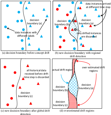
detection regions are. Considering both when and where a drift occurs is beneficial to reduce the risk of overestimating the drift regions, as shown in Figure 1.
Figure 1. For any notable concept drift, if the distribution difference is only in a small region, as shown in (b), discarding the entire historical data and retraining the learner may result in a overestimation of the drift regions, such as the red shaded regions in (d), and thereby impairing the overall performance. By contrast, regional drift detection and adaptation only address targeted regions, and will not over estimate the drifts.
To the best of our knowledge, very little research has been conducted to explicitly address concept drift by detecting and adapting to regional drifts. In one related publication, [Gama and Castillo, 2006] , the authors applied a decision tree model to detect changes in the online error-rate in each internal tree node, thereby identifying drifted nodes and updating them, respectively. The experimental results showed a good performance in detecting drift and in adapting the decision model to the new concept. Similar algorithms are in [Ikonomovska and Gama, 2008, Ikonomovska, et al., 2011, Ikonomovska, et al., 2009]. However, these algorithms mainly focus on addressing concept drift on regression problems and they all are based on decision tree models, which have limited application areas.
A detailed reviewe of other drift detection algorithms can be found in [Lu, et al., 2016]. The authors suggested to divid drift detection algorithms into three categories: 1) a statistical test monitoring raw data distribution [Lu, et al., 2016, Lu, et al., 2014]; 2) the outputs (error rates) of learners [FriasBlanco, et al., 2015], and 3) the changes of learner parameters [Su, et al., 2008]. Generally, category 1) algorithms provide a statistical significance level to ensure that detected drifts are not caused by sampling errors, but they cannot easily explain the detected drift regions. Category 2) algorithms have much less computational complexity but are not sensitive to gradual and incremental drifts. To the best of our knowledge, only one attempt at category 3) has been proposed by [Su, et al., 2008]. Their framework for modeling concept drift is creative and can be applied to many learning models. However, it is not suitable for knowledge-based learners and cannot interpret detected drifts well.
3 Local Drift Degree
In this section, we formally present the proposed test statistics, Local Drift Degree (LDD). The purpose of LDD is to quantify regional density discrepancies between two different sample sets, thereby, identifying density increased, decreased and stable regions.
-݀ The intuitive idea underlying LDD is that, given two dimensions populations 𝚨ௗ and 𝚩ௗ , if two sample sets, 𝐴 from 𝚨ௗ and 𝐵 from 𝚩ௗ , are independent and identically distributed, their local density discrepancies follow a certain normal distribtuion. Denote the feature space as 𝑉, for any 𝐴݊ subspace 𝑊 ⊆ 𝑉, it has an equality that |𝐴𝑊| 𝐵݊ / = |𝐵𝑊 | / in an ideal situation where |𝐴𝑊|,|𝐵𝑊 | represents the number 𝐵݊ , 𝐴݊ of data instances in 𝑊 that belong to 𝐴, 𝐵, and represents the total number of instances in 𝐴 and 𝐵 separately.
Definition 1. The local drift degree of a subspace 𝑊 is defined as:
Theorem 1. Given 𝚨ௗ and 𝚩ௗ have the same distribution, 𝛿𝑊~𝑁(Ͳ, 𝜎2 ), where 𝜎2 is the theoretical variance of 𝛿𝑊.
Proof. Define 𝐴𝑖 as Equation (2), and define 𝐵𝑖, 𝚨𝑖ௗ and 𝚩𝑖ௗ in the same way.
Then 𝛿𝑊 can be rewritten as Equation. (3)
Assuming 𝐴̅ contains almost all {𝐴𝑖 = ͳ} in 𝚨ௗ ̅̅̅̅, 𝐴̅ will be very closed to 𝚨ௗ ̅̅̅̅ . Therefore, 𝛿𝑊 ≈ 𝐵̅ 𝚨ௗ ̅̅̅̅ / -ͳ . In the Appendix, we have 𝐸(𝐵̅) = 𝐁ௗ ̅̅̅̅, and the expectation of 𝛿𝑊 can be acquired by Equation (4)
If 𝚨ௗ and 𝚩ௗ have the same distribution, 𝐁ௗ ̅̅̅̅ = 𝚨ௗ ̅̅̅̅ and 𝐸(𝛿𝑊) = Ͳ. According to the Central Limit Theorem, it obeys a normal distribution as it is constructed in terms of the sample average. The variance can be estimated by the Monte Carlo method. □
4 Drifted Instance Selection and Adaptation
4.1 Drifted Instance Selection
The LDD-based drifted instance selection algorithm (LDDDIS) is shown in Algorithm 1. The core idea of LDD-DIS is to use LDD to identify density decreased (𝐃ௗ ), increased (𝐃𝑖𝑛 ), and stable (𝐃𝑠𝑡 ) instances within two batches of data. The inputs are the target data batches, 𝐃1 𝐃2, the neighbourhood ratio 𝜌, and the drift significant level 𝛼.
The neighborhood ratio 𝜌 controls the size of the neighbourhood. Instead of confining the neighbourhood within a certain range, selecting the k-nearest neighbours (KNN) with a certain proportion of a data set as the neighbourhood is more robust (the k value of KNN is equal to |𝐃| ×𝜌). The reason is that KNN-based neighbourhood is independent of the shape of the feature space and is friendly to high-dimensional domains. With a proper data structure, like a binary tree, the complexity of the KNN-search can be reduced in instances data of number total the is ݊ where ,))݊(݈݃𝑂( to a sample set.
The drift significance level 𝛼 quantifies the statistical significance of concept drift. For example, in our case, if an observation is in the left tail, the system will be (ͳ -𝛼)% confidence that it is a density-decreased region. Similarly, if an observation is in the right tail, the system will be (ͳ-𝛼)% confidence that it is a density-increased region.
Without any specifications, LDD-DIS will be initialized by the default input values. LDD-DIS consists of two major steps. One is to estimate the distribution of LDD when no drift occurs, namely 𝛿′~𝒩(𝜇, 𝜎2 ), lines 1-13. The second is to compute LDD for each data instance according to the input data batches, and selects the drifted instances correspondingly, lines 14-31.
Lines 1 to 4 computes the k-nearest neighbor map of the finding for stands 𝜌) ∗ |𝐃| 𝐃, ,𝑖݀findKNN( entire data, where we 5, line at Then, 𝐃. in 𝑖݀ the (|𝐃| ∗ 𝜌) nearest neighbor of shuffle the data and resample two new batches 𝐃1′ , 𝐃2′ with the same size as 𝐃ͳ, 𝐃2. The resampling guarantees that 𝐃1′ and 𝐃2′ follow an identical distribution. As per theorem 1, consequently, the 𝛿 ′ follows 0-mean normal distribution, and the density decreasing and increasing confidence interval can be calculated by the normal inverse cumulative distribution function, as shown in lines 12, 13, denoted as norminv(𝛼, Ͳ, std(𝛿 ′)), where 𝛼 is the significance level, 0 is the mean, and std(𝛿 ′) is the estimated standard deviation. Then, we compute the LDD for each data instance according to their original distributions. For each data instance, if its LDD is less than 𝜃ௗ, it will be identified as a density decreasing instance, while if its LDD is greater than 𝜃𝑖𝑛 , it will be identified as density increasing instance, as shown in lines 14 to 31. Also, if the LDD is between 𝜃ௗ ≤ 𝛿𝑖 ≤ 𝜃𝑖𝑛, that instance will be considered as a no drift instance, or a stable instance.
| Algorithm 1: LDD Drifted Instance Selection (LDD-DIS) | |
|---|---|
| Input: | two batches of data instances, 𝐃1, 𝐃2 neighborhood ratio, 𝜌 (default 𝜌 = Ͳ.ͳ) drift significance level, 𝛼 (default 𝛼 = Ͳ.Ͳͷ) drifted data sets, 𝓓ௗ𝑟𝑖𝑡 = {𝐃1ௗ , 𝐃1𝑠𝑡 , 𝐃1𝑖𝑛 ,𝐃2ௗ , 𝐃2𝑠𝑡 ,𝐃2𝑖𝑛 } |
| Output: | |
- merge 𝐃1 and 𝐃2 as 𝐃
- 𝐃 : 𝑖݀ 2. For
- 𝜌) ∗ |𝐃| ,𝐃, 𝑖݀findKNN( = 𝐃𝑖𝑘𝑛𝑛 neighborhood, 𝑖݀ retrieve
- End
- shuffle 𝐃 and resample 𝐃1′ , 𝐃2′ without replacement
- 𝐃 : 𝑖݀ 6. For
- 𝐃1′ ∈ 𝑖݀ If
- | |𝐃𝑖𝑘𝑛𝑛∩𝐃2′ = 𝛿𝑖′ by 𝑖݀ compute the LDD of |𝐃𝑖𝑘𝑛𝑛∩𝐃1′ | -ͳ
- Else
- | |𝐃𝑖𝑘𝑛𝑛∩𝐃1′ = 𝛿𝑖′ by 𝑖݀ compute the LDD of |𝐃𝑖𝑘𝑛𝑛∩𝐃2′ | -ͳ
- End
- density decrease threshold, θௗ = norminv(𝛼, Ͳ, std(𝛿 ′))
- density increase threshold, θ𝑖𝑛 = norminv((ͳ- 𝛼), Ͳ, std(𝛿 ′))
- 𝐃 : 𝑖݀ 14. For
- 𝐃1 ∈ 𝑖݀ 15. If
- |𝐃𝑖𝑘𝑛𝑛∩𝐃𝟐| = 𝛿𝑖 by 𝑖݀ compute the LDD of |𝐃𝑖𝑘𝑛𝑛∩𝐃𝟏| -ͳ
- If 𝛿𝑖 < θௗ
- } 𝑖݀{ 18. 𝐃1ௗ = 𝐃1ௗ ∪
- Else if 𝛿𝑖 > θ𝑖𝑛
- } 𝑖݀{ 20. 𝐃1𝑖𝑛 = 𝐃1𝑖𝑛 ∪
- Else
- } 𝑖݀{ 22. 𝐃1𝑠𝑡 = 𝐃1𝑠𝑡 ∪
- Else
- |𝐃𝑖𝑘𝑛𝑛∩𝐃𝟏| = 𝛿𝑖 by 𝑖݀ compute the LDD of |𝐃𝑖𝑘𝑛𝑛∩𝐃𝟐| -ͳ
- If 𝛿𝑖 < θௗ
- } 𝑖݀{ 26. 𝐃2ௗ = 𝐃2ௗ ∪
- Else if 𝛿𝑖 > θ𝑖𝑛
- } 𝑖݀{ 28. 𝐃2𝑖𝑛 = 𝐃2𝑖𝑛 ∪
- Else
- } 𝑖݀{ 30. 𝐃2𝑠𝑡 = 𝐃2𝑠𝑡 ∪
- End
- return 𝓓ௗ𝑟𝑖𝑡 = {𝐃1ௗ ,𝐃1𝑠𝑡 ,𝐃1𝑖𝑛 ,𝐃2ௗ ,𝐃2𝑠𝑡 , 𝐃2𝑖𝑛 }
4.2 Density Synchronized Drift Adaptation
In this section, a regional drift adaptation algorithm is developed to synchronize the density discrepancies based on the identified drifted instances. The set 𝐃1ௗ , which returned by LDD-DIS, represents the data instances belonging to 𝐃1 and have decreased density compared to the set 𝐃2 . Similarly, the set 𝐃2𝑖𝑛 represents the data instances belonging to 𝐃2 and have increased density compared to data set 𝐃1. It is obvious that, if the size of 𝐃1 and 𝐃2 are the
Algorithm 2: Density Synchronized Drift Adaptation (LDD-DSDA)
Input:
Output:
𝑡݀ ,⋯,0݀ data instance arriving at each time step minimum data batch size, 𝑤 (default 𝑤 = ͳͲͲ) base learner, 𝐿 (default 𝐿 = Naive Bayes Classifier) prediction results, 𝑦̂0, ⋯, 𝑦̂𝑡
- initial 𝐃𝑡𝑟𝑖𝑛, 𝐿 = buildLearner(𝐃𝑡𝑟𝑖𝑛 )
- while stream not end, denote current time step as 𝑡
- ) 𝑡݀ ,𝐿(𝑡ܿ𝑖݀݁𝑟 3. 𝑦̂𝑡 =
- If |𝐃𝑡𝑟𝑖𝑛 | < 𝑤
- } 𝑡݀{ 5. 𝐃𝑡𝑟𝑖𝑛 = 𝐃𝑡𝑟𝑖𝑛 ∪
- Else
- } 𝑡݀{ 7. 𝐃𝑢𝑟 = 𝐃𝑢𝑟 ∪
- If |𝐃𝑡𝑟𝑖𝑛 | ≥ 𝑤 and |𝐃𝑢𝑟| ≥ 𝑤
- ݁𝑟݁𝑤ℎ 9. 𝓓ௗ𝑟𝑖𝑡 = LDD-DIS(𝐃𝑡𝑟𝑖𝑛,𝐃𝑢𝑟),
- 𝓓ௗ𝑟𝑖𝑡 = {𝐃𝑡𝑟𝑖𝑛 ௗ ,𝐃𝑡𝑟𝑖𝑛 𝑠𝑡 , 𝐃𝑡𝑟𝑖𝑛 𝑖𝑛 ,𝐃𝑢𝑟 ௗ , 𝐃𝑢𝑟 𝑠𝑡 ,𝐃𝑢𝑟 𝑖𝑛 }
- merge the detected drift regions as per Equation (5)
- based on the density of 𝐃𝑢𝑟, resample the data as 𝐃𝑡𝑟𝑖𝑛, as per Equation (6)
- build new learner, 𝐿 = buildLearner(𝐃𝑡𝑟𝑖𝑛 )
- Else
- ) 𝑡݀ 14. updateLearner(𝐿,
- End
- return 𝑦̂0, ⋯, 𝑦̂𝑡
same, then the size of 𝐃1ௗ and 𝐃2𝑖𝑛 will be the same, or is simply denoted as |𝐃1ௗ | |𝐃1| / = |𝐃2𝑖𝑛 | |𝐃2| / . This property is the foundation of the proposed density synchronized drift adaptation (DSDA) in Algorithm 2.
The intuitive idea of LDD-DSDA is to merge existing data 𝐃𝑡𝑟𝑖𝑛 with the recently buffered data 𝐃𝑢𝑟 and resample a new batch of training data 𝐃𝑡𝑟𝑖𝑛 so that the new 𝐃𝑡𝑟𝑖𝑛 has the same distribution as 𝐃𝑢𝑟 . To achieve this goal, we present the following data merging rules: 1) if no density discrepancies are detected (which means |𝐃1ௗ | |𝐃1| / = |𝐃2𝑖𝑛 | |𝐃2| / = Ͳ ) then return 𝐃𝑡𝑟𝑖𝑛 ∪𝐃𝑢𝑟 while if the unioned data set is considered redundant, return 𝐃𝑢𝑟 instead; 2) if there are regional density drifts, merging the drifted data instances as per Equation 5.
Then, to ensure the drifted regions have the same probability region drifted each in instances of subset a ,𝑟݂݂݁𝑢ܾ𝐃 density as will be resampled, denoted as 𝐃𝑠𝑚𝑝𝑙, shown as Equation 6.
where 𝐃𝑠𝑚𝑝𝑙 𝑖𝑛 are sampled from 𝐃ௗ in Equation 5. and so on.
At last replace 𝐃𝑡𝑟𝑖𝑛 by 𝐃𝑠𝑚𝑝𝑙, namely 𝐃𝑡𝑟𝑖𝑛 =𝐃𝑠𝑚𝑝𝑙
In Algorithm 2, line 1 initializes the base learner 𝐿, and line 3 uses the base learner to predict data instances arriving 4 lines From ). 𝑡݀ ,𝐿(𝑡ܿ𝑖݀݁𝑟 at the current time, denoted as to 7, the system maintains the data for training and drift detection. When both training and buffered data sets reach the minium batch size, LDD-DIS is triggered, as shown in lines 8, 9. Then the detected drift regions are synchronized, based on Equations (5), (6). Otherwise, the system incrementally ), 𝑡݀ updates the base learner, denoted as updateLearner(𝐿, shown in line 14. Finally, in line 16, the predicted labels are returned for performance analysis.
5 Experiment and Evaluation
In this section, we describe three groups of experiments to evaluate the proposed LDD. The first group examines the normality of LDD under different circumstances. The second group evaluates the LDD-DIS algorithm. Lastly, we apply the LDD-DSDA algorithm to three real-world evolving data streams and compare the results with other methods. All experiments are conducted on a 2×3.1GHz 8 core CPU 128GB RAM cluster node with unique access.
5.1 Evaluation of the Validity of LDD
Experiment 1 The distribution of LDD
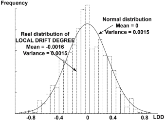
To verify the normality of LDD, two 1D data sets 𝐴, 𝐵 of equal size (5,000,000) are generated. Given a neighborhood of randomly picked points in this domain, we randomly select 10,000 points from 𝐵, and observe the number of points located in 10,000 neighborhood of points in 𝐵. This process is repeated 10,000 times to approximately describe the distribution of 𝛿. The histogram of 10,000 𝛿 is shown in Figure 2.
According to Theorem 1, LDD is normally distributed with the parameters (Ͳ, 𝑉(𝛿)). To compare the real and theoretical distribution of LDD, the line in Figure 2 represents the theoretical values of a normal distribution 𝑁(Ͳ, 𝑉(𝛿)) , where 𝑉(𝛿) stands for the variance of 𝛿.
5.2 Evaluation of LDD-DIS
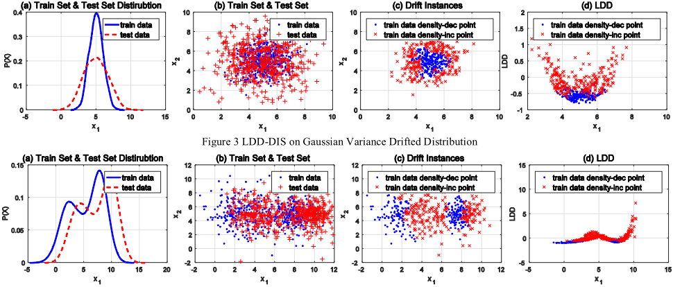
In this section, we evaluate the LDD-DIS algorithm in terms of two 2D synthetic drifted data sets. For each data set, 1,000 training cases are drawn from a specific distribution and 500 testing cases are drawn from a different distribution. We plot the estimated probability density curve of the selected feature in subfigure (a), the entire data set in subfigure (b) (blue dots represent the training set and red crosses represent the testing set), the detected drifted instances in subfigure (c) (blue dots represent decreasing density, red dots represent increasing density), and the value of LDD of the corresponding instances in subfigure (d) to demonstrate the relationship between LDD and regional density changes. The configurations of LDD are set as the default values described in Algorithm 1.
Experiment 2 Gaussian Data with Drifted Variance
This data set is generated from a bivariate Gaussian distribution. The training set has mean 𝜇 = [ͷ, ͷ] and the covariance matrix is Σ = [ͳ Ͳ Ͳ ͳ]. The testing set has the same mean vector while its covariance matrix drifts to Σ = [͵ Ͳ Ͳ ͵]. This drift forms a ring-shaped drifted region as shown in Figure 3(c).
Since the covariance of 𝑥1, 𝑥2 is 0, the patterns of drifted regions are the same from only 𝑥1 perspective. In Figure 3(a), we plot the kernel smoothing estimated density function of feature 𝑥1 for both training set (red line) and testing set (blue line). If we consider the density drift from the training set perspective, when the blue line is higher than the red line, this means in that region, the training set density is decreasing, and vice versa. Accordingly, the instances located in these regions will be identified as 𝐃𝑡𝑟𝑖𝑛 ௗ or 𝐃𝑡𝑟𝑖𝑛 𝑖𝑛 , as shown in Figure 3(c), where the red dots belong to 𝐃𝑡𝑟𝑖𝑛 𝑖𝑛 , and the blue ݊𝑖ܽ𝐃𝑡𝑟 dots belong to ௗ . The corresponding LDD value of each data instance is ploted in Figure 3(d). The higher the value of LDD, the higher the probability that this instance will drift.
Experiment 3 Mixture Distribution with Drifting Mean
To demonstrate how LDD works in a more general situation, we create a drifting Gaussian mixture data set and apply LDD to detect the drifted instances. The Gaussian mixture distribution consists of three bivariate Gaussian distributions. The three distributions for the testing set are generated based on the paramters given in Equation (7), while the testing set is generated based on the paramters given in Equation (8). The results of LDD-DIS are shown in Figure 4 with the same meaning as Figure 3.
5.3 Evaluation of LDD-DSDA
In this section, we evaluate LDD-DSDA on three real-world evolving data streams. We compare its performance to several representatives of data stream classification paradigms.
The selected comparison methods are: Hoeffding Adaptive Tree (HAT) [Bifet and Gavaldà, 2009], Accuracy Updated Ensemble (AUE) [Brzeziński and Stefanowski, 2011], SAMkNN [Losing, et al., 2016], exponentially weighted moving average charts drift detection (ECDD) [Ross, et al., 2012], and HDDM family algorithms [Frias-Blanco, et al., 2015]. All these algorithms were implemented based on the MOA framework [Bifet, et al., 2010], which is a commonly used software for evolving data stream analysis. To quantitatively evaluate LDD-DSDA, we consider the following performance metrics: accuracy (Acc.), precision (Pre.), recall (Rec.), f1-score (F1.) and computation time (Time), where Pre=TP/(TP+FP), Rec=TP/(TP+FN), and F1=2∙Pre∙Rec/(Pre+Rec). The term TP represents the number of true positive predictions, FN represents the number of false negative predictions. These metrics were evaluated in a prequential manner. To fairly compare these drift adaptation algorithms, the default parameters suggested by the authors are used, and the base classification model is set as Naïve Bayes classifier, except for SAMkNN, which is only designed for IBk classifier. The and ͳͲ = ݇ parameters for IBk classifier of SAMkNN are weighting method = uniformly weighted. Because LDDDSDA involves a random sampling process, the results may vary at different runs, we run LDD-DSDA 50 times on each data set and state the mean and standard deviation of the results. To avoid confusion on the F1-score metric, we only take the mean of Pre. and Rec. to calculate the F1 for LDDDSDA. The source code of LDD-DSDA is available at https://sites.google.com/view/anjin-concept-drift/home.
Experiment 4 Electricity Price Prediction Data Set (Elec) Elec contains 45,312 instances, collected every thirty minutes from the Australian New South Wales Electricity Market between 7 May 1996 and 5 Dec 1998. In this market, prices are not fixed and are affected by demand and supply. This data set contains eight features and two classes (up, down) and has been widely used for concept drift adaptation evaluation. We considered the classes as equally important, because both price up and down in the market is considered critical to users, and the ratio of classes is balanced, which is 58% down and 42% up. Therefore, we take the average precision (Pre.) and recall (Rec.) of both classes as the performance evaluation metrics, where average Pre = (Pre𝑙𝑠𝑠1 +Pre𝑙𝑠𝑠2 ) ʹ / , average Rec = (Rec𝑙𝑠𝑠1 + Rec𝑙𝑠𝑠2) ʹ / .
Experiment 5 Nebraska Weather Prediction Data Set (Weather)
This data set was compiled by the U.S. National Oceanic and Atmospheric Administration. It contains 8 features and 18,159 instances with 31% positive (rain) class, and 69% negative (no-rain) class. This data set was summarized by [Elwell and Polikar, 2011]. In relation to the performance metrics Pre. Rec. and F1, only the positive class (rain) is considered. This is because a correct prediction of rain is considered more important than a correct prediction of no-rain.
Experiment 6 Spam Filtering Data Set (Spam Filtering)
This data set is a collection of 9,324 email messages derived from the Spam Assassin collection. The original data set contains 39,916 features, and 9,324 emails (around 20% spam emails and 80% legitimate emails). It is commonly considered to be a typical gradual drift data set [Katakis, et al., 2009]. According to [Katakis, et al., 2009], 500 attributes were retrieved using the chi-square feature selection approach. The correct classification of legitimate emails is used to evaluate the algorithms [Katakis, et al., 2009].
Experiment Summary
As shown in Table 1, LDD-DSDA achieve the best performance in most cases. Although the execution time of LDD is slightly longer than that of the other algorithms on high-dimensional data (experiment 6), the improvement is notable. LDD-DSDA addresses a critical problem in data stream mining from a novel perspective and achieved a competitive result compared to the state-of-the-art algorithms. LDD-DSDA has the best average rank (2.33) crossing the tested data sets. Compared to the second place, which is ECDD (2.67), LDDDSDA improves the average F1 by 0.0114. According to the Friedman Test, the differences between LDD-DSDA and ECDD on Acc., Pre., Rec. and F1 are significant.
6 Conclusion and Further Study
In this paper, we analyzed existing concept drift adaptation algorithms and recognized the necessity of tracking regional drifts. Through investigating the distribution of data nearestneighbors, we proposed a novel metric, called LDD, to detect regional concept drift. Accordingly, an LDD-based density synchronization algorithm was proposed to adapt the density discrepancies. The validity of LDD and the performance of LDD-based algorithms were thoroughly evaluated using six experiments.
Acknowledgments
This work is supported by the Australian Research Coun-cil (ARC) under discovery grant DP150101645. Also, the authors would like to thank the anonymous reviewers for their valuable feedback and all members of the CAI for discussion.
A Proof of Theorem 1
To demonstrate theorem1 we introduce a random variable 𝐼𝑖
units ݊ According to the sampling techniques, selecting from N, the probability that each unit will be selected in n draws is 𝐶𝑁-1 𝑛-1 𝐶𝑁𝑛 𝑁 ݊ / = / (𝐶𝑁𝑛 is the number of n-permutations of N) and the probability that two units will be selected in n -ͳ) 𝑁(𝑁 -ͳ) ݊(݊ draws is / . Under this condition, 𝐼𝑖 satisfies the following equations:
By using 𝐼𝑖, 𝐵̅ can be rewritten by Equation. (A.3) and its expectation equals 𝐁ௗ ̅̅̅̅
̅̅̅̅
𝑁𝑖=1 = 𝐁ௗ
= 1𝑁 ∑ 𝚩𝑖ௗ
| Data Stream | #Insts | #Dim | #Class | Algorithms | Acc. | Pre. | Rec. | F1 (rank) | Time (ms) |
|---|---|---|---|---|---|---|---|---|---|
| Elec | 45,312 | 8 | 2 | LDD-DSDA HAT AUE SAMkNN ECDD HDDM-A-Test HDDM-W-Test | 0.8776±6.8E-5 0.8131 0.7544 0.7561 0.8676 0.8492 0.8409 | 0.8750±7.4E-5 0.8100 0.7514 0.7506 0.8643 0.8462 0.8374 | 0.8743±6.2E-5 0.8057 0.7408 0.74835 0.8650 0.8446 0.8367 | 0.8747 (1) 0.8078 (5) 0.7461 (7) 0.7495 (6) 0.8646 (2) 0.8454 (3) 0.8371 (4) | 1776.4±243.5 2071 3005 305082 1005 3063 1004 |
| Weather | 18,159 | 8 | 2 | LDD-DSDA HAT AUE SAMkNN ECDD HDDM-A-Test HDDM-W-Test | 0.7256±4.7E-4 0.7248 0.7243 0.7486 0.7279 0.7238 0.7282 | 0.8070±4.2E-4 0.8039 0.7862 0.6778 0.7960 0.8221 0.8018 | 0.7876±7.2E-4 0.7922 0.8217 0.3787 0.8183 0.7626 0.8021 | 0.7972 (5) 0.7980 (4) 0.8036 (2) 0.4859 (7) 0.8070 (1) 0.7912 (6) 0.8019 (3) | 982.4±177.7 2069 1006 121001 1004 1063 1004 |
| Spam Filtering | 9,324 | 500 | 2 | LDD-DSDA HAT AUE SAMkNN ECDD HDDM-A-Test HDDM-W-Test | 0.9412±4.3E-4 0.8893 0.8406 0.9247 0.8884 0.9079 0.9165 | 0.9503±5.1E-4 0.9430 0.9246 0.9227 0.9012 0.9341 0.9293 | 0.9719±4.3E-4 0.9060 0.8556 0.9809 0.9546 0.9426 0.9608 | 0.9610 (1) 0.9241 (6) 0.8888 (7) 0.9509 (2) 0.9271 (5) 0.9383 (4) 0.9448 (3) | 9942.3±746.3 5067 7012 255923 2005 2003 2003 |
@inproceedings{ijcai2017p317,
  title     = {Regional Concept Drift Detection and Density Synchronized Drift Adaptation},
  author    = {Liu, Anjin and Song, Yiliao and Zhang, Guangquan and Lu, Jie},
  booktitle = {Proceedings of the Twenty-Sixth International Joint Conference on
               Artificial Intelligence, {IJCAI-17}},
  publisher = {International Joint Conferences on Artificial Intelligence Organization},
  editor    = {Carles Sierra},
  pages     = {2280--2286},
  year      = {2017},
  month     = {8},
  note      = {Main track},
  doi       = {10.24963/ijcai.2017/317},
  url       = {https://doi.org/10.24963/ijcai.2017/317},
}
TY - CPAPER TI - Regional Concept Drift Detection and Density Synchronized Drift Adaptation AU - Liu, Anjin AU - Song, Yiliao AU - Zhang, Guangquan AU - Lu, Jie T2 - Proceedings of the Twenty-Sixth International Joint Conference on Artificial Intelligence, IJCAI-17 PB - International Joint Conferences on Artificial Intelligence Organization PY - 2017 SP - 2280 EP - 2286 DO - 10.24963/ijcai.2017/317 UR - https://doi.org/10.24963/ijcai.2017/317 ER -Copied
Machine-readable versions of this paper, for tools and AI agents:





