
CFNN: Correlation Filter Neural Network for Visual Object Tracking
Proceedings of the Twenty-Sixth International Joint Conference on Artificial Intelligence. Main track. Pages 2222-2229.
https://doi.org/10.24963/ijcai.2017/309
Keywords
- Machine Learning: Neural Networks
- Robotics and Vision: Vision and Perception
Abstract
Albeit convolutional neural network (CNN) has shown promising capacity in many computer vision tasks, applying it to visual tracking is yet far from solved. Existing methods either employ a large external dataset to undertake exhaustive pre-training or suffer from less satisfactory results in terms of accuracy and robustness. To track single target in a wide range of videos, we present a novel Correlation Filter Neural Network architecture, as well as a complete visual tracking pipeline, The proposed approach is a special case of CNN, whose initialization does not need any pre-training on the external dataset. The initialization of network enjoys the merits of cyclic sampling to achieve the appealing discriminative capability, while the network updating scheme adopts advantages from back-propagation in order to capture new appearance variations. The tracking pipeline integrates both aspects well by making them complementary to each other. We validate our tracker on OTB-2013 benchmark. The proposed tracker obtains the promising results compared to most of existing representative trackers.
- [Bertinetto et al., 2016] Luca Bertinetto, Jack Valmadre, J.F Henriques, Andrea Vedaldi, and Philip HS Torr. Fully- convolutional siamese networks for object tracking. arXiv preprint arXiv:1606.09549, 2016.
- [Bolme et al., 2010] David S Bolme, J Ross Beveridge, Bruce A Draper, and Yui Man Lui. Visual object track- ing using adaptive correlation filters. In CVPR, 2010.
- [Dalal and Triggs, 2005] Navneet Dalal and Bill Triggs. His- tograms of oriented gradients for human detection. In CVPR, 2005.
- [Danelljan et al., 2014] Martin Danelljan, Gustav Häger, Fa- had Khan, and Michael Felsberg. Accurate scale estima- tion for robust visual tracking. In British Machine Vision Conference, 2014.
- [Danelljan et al., 2015] Martin Danelljan, Gustav Hager, Fa- had Shahbaz Khan, and Michael Felsberg. Convolutional features for correlation filter based visual tracking. In ICCV Workshops, 2015.
- [Danelljan et al., 2016] Martin Danelljan, Andreas Robin- son, Fahad Shahbaz Khan, and Michael Felsberg. Beyond correlation filters: Learning continuous convolution oper- ators for visual tracking. In ECCV, 2016.
- [Deng et al., 2009] Jia Deng, Wei Dong, Richard Socher, Li- Jia Li, Kai Li, and Li Fei-Fei. Imagenet: A large-scale hierarchical image database. In CVPR, 2009.
- [Felzenszwalb et al., 2010] Pedro F Felzenszwalb, Ross B Girshick, David McAllester, and Deva Ramanan. Object detection with discriminatively trained part-based models. IEEE TPAMI, 32(9):1627-1645, 2010.
- [Gao et al., 2014] Jin Gao, Haibin Ling, Weiming Hu, and Junliang Xing. Transfer learning based visual tracking with gaussian processes regression. In ECCV, 2014.
- [Held et al., 2016] David Held, Sebastian Thrun, and Silvio Savarese. Learning to track at 100 fps with deep regression networks. In ECCV, 2016.
- [Henriques et al., 2015] J.F Henriques, Rui Caseiro, Pedro Martins, and Jorge Batista. High-speed tracking with ker- nelized correlation filters. In IEEE TPAMI, volume 37, pages 583-596, 2015.
- [Kiani et al., 2013] Hamed Kiani, Terence Sim, and Simon Lucey. Multi-channel correlation filters. In ICCV, 2013.
- [Kristan et al., 2015] Matej Kristan, Jiri Matas, Ales Leonardis, Michael Felsberg, Luka Cehovin, Gustavo Fernandez, Tomas Vojir, Gustav Hager, Georg Nebehay, and Roman Pflugfelder. The visual object tracking vot2015 challenge results. In ICCV Workshops, 2015.
- [Krizhevsky et al., 2012] Alex Krizhevsky, Ilya Sutskever, and Geoffrey E Hinton. Imagenet classification with deep convolutional neural networks. In F. Pereira, C. J. C. Burges, L. Bottou, and K. Q. Weinberger, editors, Ad- vances in Neural Information Processing Systems 25, pages 1097-1105.
- Curran Associates, Inc., 2012.
- [Li and Zhu, 2014] Yang Li and Jianke Zhu. A scale adaptive kernel correlation filter tracker with feature integration. In ECCV Workshops, 2014.
- [Li et al., 2015] Yang Li, Jianke Zhu, and Steven CH Hoi. Reliable patch trackers: Robust visual tracking by exploit- ing reliable patches. In CVPR, 2015.
- [Li et al., 2016] Hanxi Li, Yi Li, and Fatih Porikli. Deep- track: Learning discriminative feature representations on- line for robust visual tracking. IEEE TIP, 25(4):1834- 1848, 2016.
- [Liu et al., 2015] Ting Liu, Gang Wang, and Qingxiong Yang. Real-time part-based visual tracking via adaptive correlation filters. In CVPR, 2015.
- [Nam and Han, 2016] Hyeonseob Nam and Bohyung Han. Learning multi-domain convolutional neural networks for visual tracking. In CVPR, 2016.
- [Nguyen et al., 2002] Hieu Tat Nguyen, Marcel Worring, Rein Van Den Boomgaard, and Arnold WM Smeulders. Tracking nonparameterized object contours in video. IEEE TIP, 11(9):1081-1091, 2002.
- [Sung and Poggio, 1998] K-K Sung and Tomaso Poggio. Example-based learning for view-based human face detec- tion. IEEE TPAMI, 20(1):39-51, 1998.
- [Tao et al., 2016] Ran Tao, Efstratios Gavves, and Arnold W. M. Smeulders. Transfer learning based visual tracking with gaussian processes regression. In CVPR, 2016.
- [Van De Weijer et al., 2009] Joost Van De Weijer, Cordelia Schmid, Jakob Verbeek, and Diane Larlus. Learning color names for real-world applications. IEEE TIP, 18(7):1512- 1523, 2009.
- [Vedaldi and Lenc, 2015] A. Vedaldi and K. Lenc. Matcon- vnet -convolutional neural networks for matlab. In ACM International Conference on Multimedia, 2015.
- [Wang and Yeung, 2013] Naiyan Wang and Dit-Yan Yeung. Learning a deep compact image representation for visual tracking. In Advances in Neural Information Processing Systems, 2013.
- [Wang et al., 2015] Lijun Wang, Wanli Ouyang, Xiaogang Wang, and Huchuan Lu. Visual tracking with fully con- volutional networks. In ICCV, 2015.
- [Wu et al., 2013] Yi Wu, Jongwoo Lim, and Ming-Hsuan Yang. Online object tracking: A benchmark. In CVPR, 2013.
- [Zhang et al., 2014] K. Zhang, L. Zhang, Q Liu, D. Zhang, and M.-H Yang. Fast visual tracking via dense spatio- temporal context learning. In ECCV, 2014.
- [Zhang et al., 2015] Kaihua Zhang, Qingshan Liu, Yi Wu, and Ming-Hsuan Yang. Robust visual tracking via con- volutional networks. arXiv preprint arXiv:1501.04505, 2015.
- [Zhou et al., 2007] Xue Zhou, Weiming Hu, Ying Chen, and Wei Hu. Markov random field modeled level sets method for object tracking with moving cameras. In Asian Con- ference on Computer Vision, 2007.
References were extracted automatically from the PDF and may contain errors.
Full text extracted automatically from the PDF; figures, tables and equations may differ. The PDF is the version of record.
1 Introduction
Although visual tracking plays a fundamental role in computer vision community, it is not yet a well-solved problem due to many challenges. One difficulty is the diversity of targets to be tracked in videos. While some methods [Nguyen et al., 2002; Zhou et al., 2007] focus on certain tracking situations, a generally applicable approach could be more useful considering the emergence of different kinds of videos from real world. Another main challenge is the appearance variations of the targets. Due to illumination changes and scale variations, out-of-plane rotation, occlusion and deformation, it could be cumbersome to track the specific object through a long video sequence according to ground truth in a frame.
∗Equal contributions. This work was done when Mr. Zhan Xu was a visiting student at Zhejiang University.
†Corresponding author.
Recently, correlation filter-based methods [Bolme et al., 2010; Henriques et al., 2015; Li and Zhu, 2014; Danelljan et al., 2014; Liu et al., 2015; Zhang et al., 2014] have shown high robustness in tracking different types of targets. They usually learn filters to regress a Gaussian map in Fourier domain, in which the process can be extremely efficient through the given video. To solve the problem of appearance variations, they employ a linear combination of the learned model in current frame and the ones from previous frames with corresponding weights. The most common weights used in the literature [Bolme et al., 2010; Danelljan et al., 2014] are exponentially decaying, which is quite straightforwad in implementation. However, it does not integrate the most important information, e.g. hard negative samples, from all frames in a reasonable manner.
On the other hand, deep learning has achieved remarkable performance in many computer vision tasks such as image classification [Krizhevsky et al., 2012]. More and more works start to focus on employing Convolution Neural Network (CNN) in visual object tracking [Wang and Yeung, 2013; Li et al., 2016; Wang et al., 2015; Nam and Han, 2016; Zhang et al., 2015; Held et al., 2016; Tao et al., 2016; Bertinetto et al., 2016; Danelljan et al., 2016]. To obtain better generalization capability, many previous approaches such as [Nam and Han, 2016; Held et al., 2016] try to train their models with a tremendous amount of videos (sometimes also use images), which leads to heavy computational workload. Collecting enough labeled samples is difficult, and training a model with them usually needs much time and careful tuning in order to achieve satisfactory performance.
With observation of the similarity between correlation filter operation and deep learning convolutional operation, we believe that there is an implicit relationship between correlation filter and CNN, since they both concentrate on finding good filters to distinguish foreground object from background. One merit of correlation filter-based method is to quickly learn a model from single frame without the need of training on extra dataset, which can be used as a beneficial complement for CNN-based approach.
In this paper, we present a novel Correlation Filter Neural Network (CFNN) tracker with the advantages of both deep learning methods and correlation filter-based methods. The proposed approach follows the deep learning trackers' framework meanwhile does not need any pre-training. To this end, we densely sample the first frame with circulant matrix, and apply ridge regression to calculate an approximate model to the proposed network. By integrating the model into a twolayer CNN structure, our method can be initialized efficiently. Secondly, the proposed network is designed to output a target location probability map can be utilized to collect negative samples easily. This gives the proposed method an ability to update the model selectively. Finally, when reaching a certain interval, we use the samples collected along the way to tune the CFNN with back propagation, which updates its weights adaptively to the variation of appearance. The experimental results show that our method performs competitively compared to other tracking methods.
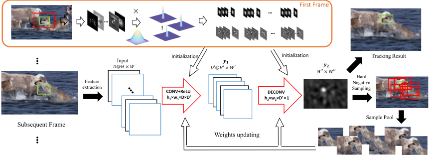
The main contributions of this work are summarized as follows: 1) A novel CFNN architecture for visual tracking. Unlike traditional deep learning based trackers [Held et al., 2016; Nam and Han, 2016] which regress the coordinates of the object in the frame, the proposed network outputs a target location probability map. The maximal value of this probability map indicates the new position of target; 2) A fast approach for the initialization of the proposed CFNN. With a quite simple architecture, our network can be constructed without pre-training. This greatly alleviates the burden of collecting a large set of external data and helps training the model from scratch; 3) A complete tracking pipeline which takes the feature map as input and a probability map as output. During the process of tracking, the weights of CFNN are also updated in this pipeline to adapt to new target's appearance; 4) The full implementation is publicly available 1 .
2 RelatedWork
In this section, we briefly review the most relevant visual tracking methods including correlation filter-based trackers and CNN-based methods.
2.1 Correlation Filter Tracker
[Bolme et al., 2010] formulate the filter learning as a regression problem which estimates the filter by minimizing overall cost according to samples from the first frame. [Henriques et al., 2015] suggest that surprisingly favorable results for ridge regression can be achieved by sampling densely with circulant matrix and utilizing features like Histogram of Oriented Gradients (HOG) [Dalal and Triggs, 2005] using kernel trick. Many extensions of correlation filter-based tracking are proposed afterwards. For example, [Li and Zhu, 2014; Danelljan et al., 2014] cope with scale estimation. Moreover, [Liu et al., 2015; Li et al., 2015] introduce the partbased tracking strategy. [Danelljan et al., 2016] propose an interpolation method to merge convolutional maps from multiple layers in order to obtain much reliable response map.
1 https://github.com/enderhsu/CFNN
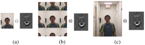
By taking advantage of the CNN method, the proposed approach avoids two defects of them. First, correlation filterbased trackers employ dot-product in frequency domain to obtain the correlation result, which is equivalent to correlation in time domain with circulant padding around original searching window. Since the template has the same size as the searching window, a large area of circulant padding may introduce the unnecessary boundary effects, as shown in Fig. 3(a) and Fig. 3(b). Second, the updating strategy for most of correlation filter-based trackers is relatively na¨ıve. Thus, it may fail to grasp and integrate the most important information from all the previous frames well. With different updating strategy, our approach introduces hard negative sampling and achieves better results.
2.2 Convolutional Neural Network Tracker
Most of CNN-based methods focus on how to extract good features with CNN to better represent the target. They train a pre-built target model before the tracking. [Wang and Yeung, 2013] emphasize on feature representation with CNN. Discrimination is performed by a classification layer. [Wang et al., 2015] utilize two layers from VGG net, a lower layer and a top layer, to represent the target from two aspects, which employ a principled strategy to discard noisy or unrelated feature maps. [Zhang et al., 2015] propose a simple CNN to exploit local geometric information and distinguish background patches from foreground ones. [Held et al., 2016] utilize a large number of labeled videos as well as images from ImageNet [Deng et al., 2009] to train a network offline. Such a network can be used to track various targets without the need of online updating. Several approaches [Nam and Han, 2016; Tao et al., 2016; Bertinetto et al., 2016] try to exploit the different CNN architecture for visual tracking. Multi-domain learning algorithm in [Nam and Han, 2016] shares common network layers at feature extraction with different videos and proceeds their own fully-connected layers later. Moreover, Siamese networks [Tao et al., 2016; Bertinetto et al., 2016] seek the relationship between two sequential frames to locate the target.
Compared with CNN-based trackers, the proposed CFNN emphasizing on discriminative classification without pretraining on external dataset. With the particular two-layer CNN architecture, our model can be trained efficiently with a few samples. In addition, conventional CNN-based trackers need the fixed size input and output coordinates of a single location which is inefficient. Our approach is able to extend the searching area to arbitrary size easily and effectively.
3 ProposedMethod
3.1 Architecture of Proposed Neural Network
In contrast to the traditional CNN-based tracking approaches, our presented CFNN focuses only on how to identify the target from background area. We find that a lightweight twolayer architecture is sufficient for this purpose. Such twolayer architecture shrinks the volume of our tracker while releasing the burden for large-scale initialization. Mathematically, our tracking process takes the following form:
where x is an image patch and F(·) represents features extraction operator. We use f1, f2 to denote the first and second layer of our network, respectively. The output P(x) is the response map of the input image patch. Each value in P(x) denotes the probability of that position being the center of the target.
The first layer f1 obtains the response maps with multiple filters. Suppose each F(x) ∈ RH×W×D contains D channels. In this layer, we construct D′ filters, denoted by w1 = w1 1 , w2 1 , ...wD′ 1 , to perform convolution with the input feature. Suppose w1 ∈ Rh1×w1×D×D′ where h1 × w1 is the kernel size. After the convolution operation, we have first-layer output map y1 = f1(F(x)) ∈ RH′×W ′×D′ where the i-th channel yi1 = f i1 = σ(F(x) ⊗wi1 + b1). ⊗ indicates the convolutional operator and σ(·) is a ReLU activation function.
The second layer f2 merges response maps yi1 from the first layer in a reasonable way, and exploits the deconvolution to raise the resolution of final response map. Suppose w2 ∈ Rh2×w2×D′×1 with a fractional stride, deconvolution is performed by f2 yields y2 ∈ RH′′×W ′′×1 (H′′ > H′ ,W ′′ > W ′ ), which is the final probability map from CFNN. The overall structure of our proposed CFNN is illustrated in Fig. 1.
We aim to train the weights in both layers based on training samples sj . The samples sj = F(xj ) consist of feature maps of the cropped patches from frames in the same sequence. The loss of our CFNN is defined as follows:
where M is the total number of samples and w = [w1,w2] denotes all parameters in the network. ti represents the desired probabilty map. It is generated with a Gaussian-like distribution indicating the position of the target in the original image. λ is a weight parameter to prevent overfitting.
3.2 Weights Initialization
In terms of tracking, it is impractical to train a CNN from scratch due to the relative small number of available samples extracted from a single frame.
We address such a problem by taking a more controllable route. For notation simplicity, we suppose there is only single filter in the first layer. We temporally ignore the second layer for fast computation, i.e. f2(x) = x. Also, we will focus on single-channel input feature map, which will be extended to multiple channels later. This simplifies our whole model into a convolution operator in 2D. Then, Eq. 2 can be rewritten into the following form:
where b1 is a small bias in the first layer. We intend to find the optimal w1 that minimizes the above equation. Because of non-linear operation σ(·), the Eq.3 is not easy to be optimized. Instead, we solve the following minimization equation:
Where t′i = ti -b1 and ⋆ indicates the correlation operation. ˜w1 is the flipping verison of w1 because of the slight difference of correlation and convolution. According to the definition, ReLu(x) = max(0, x), ReLu(x) = x when x > 0. We assume si ⊗ w1 + b1 > 0, since Eq. 3 is regressed to a Gaussian like response map and the negative value is useless. As we only need a rough initialization of w1 and ReLU is ReLu(x) = x when x >= 0, such approximation is reasonable. Following [Kiani et al., 2013], we formulate the calculation of w1 in Fourier domain, where w1 can be easily calculated in the closed-form:
(c)
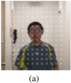
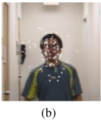
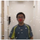
Figure 2: Three sampling approaches we tested. (a) Uniformly sampling with fixed interval. (b) Random sampling according to the normal distribution. (c) Random sampling according to the uniform distribution. Approach (c) obtains the best results.
where matrix ˆSi = [dv(ˆs1i )T , dv(ˆs2i )T , ..., dv(ˆsDi )T ] and dv(·) = diag(vec(·)). ˆ· is the Discrete Fourier transform. I represents an identity matrix.
As shown in [Henriques et al., 2015], when dealing with one image frame, the weights w1 in Fourier domain can be calculated efficiently with cyclic shift and convolution theorem as below:
where s0 is the feature map extracted from the image patch. We follow [Henriques et al., 2015] for the optimization.
Parameter λ′ controls the importance of regularization imposed on the regression. Selecting different λ′ has effects on performance of the calculated filter w1. To make our tracker more robust, we employ a set of different λ′ in our model. Then, w1 becomes an array of multiple kernels w1 1 , w2 1 , ...wD′ 1 . Accordingly, the depth of y1 also increases to D′ , where each channel is a response map obtained by kernel wi1 .
So far we have omitted the second layer by assuming f2(x) = x. When we extract feature map from the original image patch, the resolution always falls due to local context summarization (HOG) or pooling (CNN). This losses the pixel-wise accuracy during tracking. To alleviate this problem, we further extend the receptive field of w2 (7 × 7 in our experiment) to make the second layer of our CFNN into a deconvolutional layer. By this means, f2 not only merges yi1 , but also raises the resolution of our final response map. Each channel of w2 is initialized according to a Gaussian distribution with a maximal value 1/D′ in the center. Small random number is also added to each weight of w2 to introduce randomness for weights adjustment. Positions with larger distance to the center have less weights. Thus, each final response is made of multiple responses from y1 while emphasizing on those with better correspondence.
3.3 Weights Updating
After the initialization, we adopt the conventional backpropagation to update the weights during the tracking process and enrich our sample pool by applying hard negative mining method [Sung and Poggio, 1998] to take in more challenging samples. According to a normal distribution with large standard deviation, we collect a few sample patches in a wider range. By adopting forward propagation, we can obtain the final probability maps for these patches. Comparing them with the tracking result, we discard half of sample patches with relatively small resulting deviations, and put the other half into our sample pool as hard samples.
The updating process will stop once a maximal number of iteration is reached. Moreover, we adopt an early-stop strategy, which aims to accelerate the tuning process by omitting unnecessary iterations. To this end, we record the cost from all iterations, denoted as L1, L2, ..., Ln, where n is the current iteration. If the following two conditions are both met, we immediately terminate the updating process without reaching the maximal iteration number: 1) reach 3/4 of the
is a testing interval length (typically 4). θ is the ratio threshold to determine whether the last few times of iteration are important and whether we need more iteration. We set it to 0.98 empirically.
We employ an automatic adjustment measure to handle the exception during updating. Generally, the exception during updating can be detected when the cost defined in Eq. 2 from two sequential iterations increases dramatically. After each tuning iteration, we calculate the cost for the current network, and compare it with the cost from last iteration. If the ratio between these two costs is larger than a threshold, we regard it as an exception and launch the handling measure: 1) discard all the weights modification during this iteration and reset the status of all layers to that from last iteration; 2) decrease the learning rate to half of the original one to avoid network collapse raised by large learning rate. Once the learning rate is reduced, we start to increase it in a tender manner. We raise it 1.07 times larger at each iteration until reaching the original learning rate. Keeping the learning rate dynamic and flexible ensures the updating process to be robust to various scenarios.
3.4 Tracking Framework
For our proposed two-layer CNN tracking scheme, the target is localized by maximizing the confidence score with the probability maps. Formally, the center location of the target is determined as follows:
where z denotes the location of the target in a query frame. P(˜z) denotes the probability map which indicates the probability that each point is the target center. x defines a searching space with potential candidates. c is the prior constraint extracted from all the previous frames.
In our tracking system, priori constraint c is embedded in the weights of our network since samples from each previous frames are used to adjust the weights. With the learnt CNN, tracking process is formulated as forward propagation. For any position in a searching window, the probability of this position being the target's center can be obtained by passing its surrounding patch into our system as Eq. 2.
Specifically, we crop a search window to locate the target before tracking around the bounding box of the target from the previous frame. Then, we generate the feature map from the search window by extracting proper features, and multiply a Hann window with it. We employ such manipulated feature map as the input of our two-layer convolutional neural network. Our CFNN tracker performs tracking for the subsequent frames by forward propagation, and predicts the position of the target. During the tracking process, we collect a set of samples from the each frame, and generate their corresponding labels based on prediction as well. We adjust the weights of the CNN every update interval frames to take new appearance variation into account. The whole algorithm is illustrated in Algorithm 1.
4 Experiments
In this section, we give the details on our implementation and perform comparisons with other trackers on the benchmark.
4.1 Experimental Setup
We implement our proposed CFNN tracker in Matlab without further optimization. The CNN part is built on MatConvNet toolkit [Vedaldi and Lenc, 2015]. We conduct all the experiments on a PC with Intel(R) core(TM) i7-4790K 4.00GHz CPU, 32G RAM and a NVIDIA GTX TITAN graphics card.
Feature Selection: In our work, we adopt two kinds of handcrafted features to represent the target, HOG [Felzenszwalb et al., 2010] and color naming [Van De Weijer et al., 2009]. These two features are concatenated together to form a high-dimensional feature map.
Feature extraction is not presented as a layer in our convolutional neural network. Theoretically, we can employ any type of feature as long as it can represent the image context. We notice that some CNN-based trackers [Wang and Yeung, 2013; Danelljan et al., 2016; 2015] employ convolutional feature for tracking. Such a feature extraction can be used as input to our CFNN alternatively, which can be achieved by putting additional convolutional layers ahead of our CFNN and concatenate them together. However, as we mentioned, such convolutional feature more or less involves pre-training on external data.
Other Parameters: We employ the same parameters as [Henriques et al., 2015] in feature extraction. For each input patch, we can get a 31-channel feature map whose size is about 1/4 of the original patch. Thus, h1 and w1 is also 1/4 of the original patch. To extract color naming feature with the same spatial size, we first resize the image patch into the same size as the HOG feature map, and then convert it into color space. Thus, both feature maps can be concatenated together. For color image, we eventually obtain a 42-channel feature Algorithm 1 CFNN: the Correlation Filter Neural Network tracker
Require:
Ground truth z0 at the first frame;
Ensure:
The CFNNmodel f2 ◦ f1(F(x)) for tracked target;
The new target state, zk (k = 1, 2, ...);
- 1: Initialize weights in f1 according to Eq. 6 based on x0 and put small Gaussian filters in f2;
- 2: for every sub-sequential observation xk do
- 3: Generate observation xik at several different scales;
- 4: Perform forward propagation with xik to get P(xik) = f2 ◦ f1(F(xik));
- 5: Determine zk according to Eq. 7;
- 6: Randomly select samples si in the same frame around zk and generate ideal convolutional target ti;
- 7: if k%update interval == 0 then
- 8: while less thanmax iter and not reach early-stop conditions do
- 9: Update the model with si and ti according to Eq. 2;
- 10: Discard current si, ti;
- 11: end while
- 12: end if
- 13: end for
and D = 42. For gray image, we get a 33-channel one and D = 33. Accordingly, the second layer of our CFNN tracker has filter size h2×w2×D′ ×1 = 7×7×5×1 with a stride of 1/4, which will raise the resolution back to the original level.
Both the input patch for initializing weights and the rectangular searching area are set 2.5 times as large as the target bounding box with the same height-width proportions. The standard derivation of Gaussian distribution used for generating convolutional target is determined by the size of target in the response map. That is, we re-scale the original image patch to have the same resolution with its feature map, and multiply the scaled target size with a fixed factor (0.1 in this work) to get the standard derivation.
The first layer of CFNN has multiple filters generated from different λ′ . In our experience, we sample five λ′ as [0.25 0.5 1 2 4]×1e-4. In addition, we apply a multiple scale search strategy as [Li and Zhu, 2014] with scaling pool, [0.985 0.99 0.995 1 1.005 1.01 1.015]. For sample collection, we select 80 samples per frame including 65 regular samples and 15 hard negative samples. For weights updating, we perform tuning every 15 frames during the first 160 frames and every 20 frames during later frames. The learning rate is set to 3e-4. Batch size is set to 80, and the maximal iteration number is set to 20. We also set a momentum of 0.8 in order to accelerate the convergence. All parameters are chosen empirically and our matlab code runs at 1 fps. Please note the implementation is quite naive. A multi-thread version can be easily achieved and runs much faster.
4.2 Experiment on OTB-2013
We evaluate the performance of the proposed approach on OTB-2013 [Wu et al., 2013] which consists of 50 sequences with different attributes, such as illumination variation, outof-plane rotation, blur, occlusion and deformation. Since OTB-2013 is regarded as the most representative indicator of tracking performance, we conduct comparison with some state-of-the-art trackers including SAMF [Li and Zhu, 2014], DSST [Danelljan et al., 2014], KCF [Henriques et al., 2015], DLT [Wang and Yeung, 2013] and TGPR [Gao et al., 2014] as well as all the 29 trackers contained in the tracking benchmark toolkit 2 . The results of additional trackers are either provided by the authors on their websites or obtained with their raw codes with the default setting.
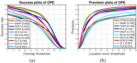
Fig. 4 shows the overall VOR and CLE curves. To make it clear, we only show the top ten trackers. With both metrics, our proposed tracker achieves the best performance with a score of 0.595 on success plot and 0.803 on precision plot. Specifically, our proposed tracker outperforms DLT at a large margin. Note that DLT is the representative approach for CNN-based tracking, who can only achieves 0.436 and 0.587 on both plots. On the other hand, our approach achieves 4% to 10% performance improvement over baseline KCF and its variants. This indicates that our approach does not lose fine properties from conventional correlation filter-based trackers. The proposed CFNN framework with the weights updating strategy, prominently improves the previous methods.
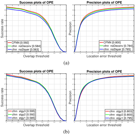
Fig. 5(a) shows the comparison plot of different network architecture on OTB-2013 dataset to illustrate the effect of each layer in our CFNN tracker. The first network, denoted as cfnn no2layer, only has the first layer of our CFNN (including ReLU layer). This layer consists of a single filter (with λ′ = 0.0001) to ensure the output has single channel. cfnn no2layer can be viewd as a CF based tracker with a back-propagation updating strategy. The second network, denoted as cfnn noDeconv, is slightly improved by adding a second layer. This enables us to put multiple filters in the first layer with different λ′ . However, w2 is a 1 × 1 ×D′ filter and each value is assigned as 1/D′ . This means we omit deconvolution with cfnn noDeconv. Intuitively, cfnn noDeconv can be viewed as a fusion of different CF based trackers with different λ settings and back-propagation updating strategy. CFNN is the comphrensive version of our proposed method. Please note that all parameters are same thorough these three architectures. From these experimental results, we can see that multiple filters performs better than single filter in the first layer, and the deconvolution helps to improve the performance of our tracker.
Sampling is performed after the target position is confirmed in each frame. We first pick some sample seeds randomly around the predicted target position. We tried three sampling methods as illustrated in Fig. 2, and the best performance is achieved when all sample seeds obey uniform distribution. Fig. 5(b) is the comparison plot among different sampling strategy, as mentioned in Fig. 2. cfnn stgy1 samples with uniform interval (Fig. 2(a)). cfnn stgy2 samples according to normal distribution with target's center as mean position (Fig. 2(b)). cfnn stgy3 samples according to uniform distribution (Fig. 2(c)). We can see that cfnn stgy3 performs slightly better than cfnn stgy2, while both works obviously better than cfnn stgy1. We employ cfnn stgy3 in all the experiments.
2 http://cvlab.hanyang.ac.kr/tracker benchmark
4.3 Experiment onMore Sequences
In this experiment, we evaluate our proposed tracker on a certain type of sequences - those who have dramatic target or camera movement. Such type of videos are very challenging for tracking as they always demonstrate strong motion blur, in-plane and out-of-plane rotation and large-margin position changes. It occurs extensively when video is captured by handheld devices or at sports events.
Our proposed tracker can handle such type of sequences much better than existing approaches, which has been partially proved in the last experiment. This is mainly because the proposed CFNN framework is able to adjust the layer weights to better distinguish foreground from background, and emphasize on the most decisive response maps. Besides, forward convolution in our CFNN enables valid tracking in a larger area without introducing boundary interference.
We select 10 sequences from previous study [Kristan et al.,
| mean VOR | crossing | biker | girl | ball | pedestrian | dog | blurCar | human2 | handball | man | avg. | |
|---|---|---|---|---|---|---|---|---|---|---|---|---|
| TGPR | 0.5385 | 0.2855 | 0.0571 | 0.8034 | 0.3245 | 0.6498 | 0.7501 | 0.1950 | 0.0687 | 0.2785 | 0.3951 | |
| KCF | 0.5132 | 0.2495 | 0.1060 | 0.4705 | 0.1659 | 0.5632 | 0.8107 | 0.1766 | 0.1456 | 0.8312 | 0.4032 | |
| DSST | 0.7109 | 0.2745 | 0.0952 | 0.3892 | 0.1904 | 0.0650 | 0.8418 | 0.4144 | 0.0626 | 0.8430 | 0.3887 | |
| ASLA | 0.3848 | 0.3851 | 0.0663 | 0.1066 | 0.7240 | 0.7526 | 0.1859 | 0.6658 | 0.1035 | 0.8256 | 0.4200 | |
| SAMF | 0.6416 | 0.2456 | 0.6180 | 0.8319 | 0.1741 | 0.6838 | 0.8465 | 0.6666 | 0.0694 | 0.8558 | 0.5633 | |
| DLT | 0.6785 | 0.5211 | 0.0621 | 0.1858 | 0.1672 | 0.0482 | 0.1124 | 0.7495 | 0.0245 | 0.7725 | 0.3322 | |
| Struck | 0.4988 | 0.4990 | 0.1712 | 0.4637 | 0.3001 | 0.3531 | 0.3126 | 0.6808 | 0.1347 | 0.8895 | 0.4304 | |
| CFNN | 0.6425 | 0.3527 | 0.6529 | 0.8388 | 0.3621 | 0.7066 | 0.8279 | 0.7034 | 0.2441 | 0.8790 | 0.6210 | |
| TGPR | 20.2208 | 99.5222 | 291.2551 | 4.0798 | 4.1192 | 4.2658 | 8.3578 | 123.6110 | 73.3868 | 17.4529 | 64.6271 | |
| KCF | 14.7956 | 71.1610 | 140.2529 | 53.4102 | 242.7280 | 8.0368 | 4.1388 | 107.4042 | 30.7153 | 2.2557 | 67.4899 | |
| DSST | 8.7464 | 69.0021 | 128.3205 | 79.5626 | 234.1737 | 272.3239 | 3.2676 | 102.4550 | 60.9645 | 1.5111 | 96.0327 | |
| mean ASLA | 43.6852 | 78.9530 | 328.4980 | 95.4083 | 4.2541 | 6.1981 | 71.1535 | 21.4405 | 27.8917 | 1.7759 | 67.9258 | |
| CEL SAMF | 12.2718 | 74.6270 | 38.9573 | 3.4618 | 227.2136 | 5.7376 | 3.5831 | 21.9038 | 75.7324 | 1.8067 | 46.5295 | |
| DLT | 15.6529 | 10.7380 | 290.8835 | 185.0039 | 250.4971 | 331.3163 | 141.2786 | 19.7233 | 59.6693 | 1.5132 | 130.6276 | |
| Struck | 19.3409 | 4.3421 | 137.4185 | 63.1518 | 6.0217 | 7.4616 | 50.4882 | 23.9734 | 18.8602 | 1.7304 | 33.2789 | |
| CFNN | 6.1341 | 60.6947 | 33.4082 | 3.0803 | 9.5459 | 4.7049 | 3.5332 | 19.4547 | 34.4594 | 1.3718 | 17.6387 |
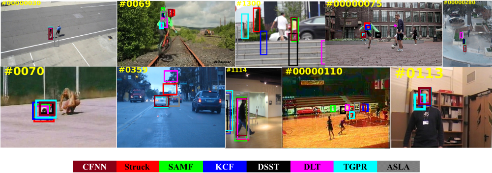
2015] and [Wu et al., 2013]. All these sequences are different from those in OTB-2013, and all contain the dramatic movement. We also choose another 8 trackers ranking among top-10 (in terms of AUC score) in last experiment for comparison. As illustrated in Fig. 6, such challenge makes many previous methods drift away. On the contrary, our tracker sticks at those targets firmly and shows quite robust performance against frame shaking and blur.
Specifically, the focal length of the camera change in Girls, bringing blur in some frames. Besides, the target girl moves extensively in the sequence, and is occluded by other people several times. KCF, Struck and DSST fail to locate the target in such situation and drift away. In BlurCar, the camera shakes which makes the capturing angle changes dramatically and bring blur. In Human, target moves and demonstrates much deformation. These cause failure for other trackers while our tracker successfully tracks the target.
Table 1 lists the the mean VOR score and the mean CEL error of each sequences obtained by different approaches. On such type of sequences, our tracker shows great potential by improving conventional tracking results at a large margin.
5 Conclusion and FutureWork
In this paper, we propose a correlation filter neural network tracking approach, which enjoys the merits of both correlation filter and deep learning. Our presented approach does not need pre-training on the external dataset. All weights in CFNN are initialized by calculating a ridge regression merely according to the ground truth in the first frame. Hence, the architecture of the CFNN is simple while retaining the advantage of correlation filter-based trackers. Under the proposed CFNN framework, we introduce a complete tracking pipeline, which continuously collects samples and updates all weights to adapt to the new appearance variation. We evaluate our tracking approach on OTB-2013 dataset and some other challenging sequences, as well as comparing with some representative trackers. Experiments show that our tracking approach achieves comparable and promising results. We believe our proposed approach can be a beneficial complement for the visual tracking community.
Acknowledgments
This work is supported by the National Key Research and Development Program of China (No. 2016YFB1001501).
@inproceedings{ijcai2017p309,
  title     = {CFNN: Correlation Filter Neural Network for Visual Object Tracking},
  author    = {Li, Yang and Xu, Zhan and Zhu, Jianke},
  booktitle = {Proceedings of the Twenty-Sixth International Joint Conference on
               Artificial Intelligence, {IJCAI-17}},
  publisher = {International Joint Conferences on Artificial Intelligence Organization},
  editor    = {Carles Sierra},
  pages     = {2222--2229},
  year      = {2017},
  month     = {8},
  note      = {Main track},
  doi       = {10.24963/ijcai.2017/309},
  url       = {https://doi.org/10.24963/ijcai.2017/309},
}
TY - CPAPER TI - CFNN: Correlation Filter Neural Network for Visual Object Tracking AU - Li, Yang AU - Xu, Zhan AU - Zhu, Jianke T2 - Proceedings of the Twenty-Sixth International Joint Conference on Artificial Intelligence, IJCAI-17 PB - International Joint Conferences on Artificial Intelligence Organization PY - 2017 SP - 2222 EP - 2229 DO - 10.24963/ijcai.2017/309 UR - https://doi.org/10.24963/ijcai.2017/309 ER -Copied
Machine-readable versions of this paper, for tools and AI agents:





