
Classification and Representation Joint Learning via Deep Networks
Proceedings of the Twenty-Sixth International Joint Conference on Artificial Intelligence. Main track. Pages 2215-2221.
https://doi.org/10.24963/ijcai.2017/308
Keywords
- Machine Learning: Feature Selection/Construction
- Machine Learning: Classification
Abstract
Deep learning has been proven to be effective for classification problems. However, the majority of previous works trained classifiers by considering only class label information and ignoring the local information from the spatial distribution of training samples. In this paper, we propose a deep learning framework that considers both class label information and local spatial distribution information between training samples. A two-channel network with shared weights is used to measure the local distribution. The classification performance can be improved with more detailed information provided by the local distribution, particularly when the training samples are insufficient. Additionally, the class label information can help to learn better feature representations compared with other feature learning methods that use only local distribution information between samples. The local distribution constraint between sample pairs can also be viewed as a regularization of the network, which can efficiently prevent the overfitting problem. Extensive experiments are conducted on several benchmark image classification datasets, and the results demonstrate the effectiveness of our proposed method.
- [Breiman, 2001] Leo Breiman. Random forests. Machine learning, 45(1):5-32, 2001.
- [Cheng et al., 2016] De Cheng, Yihong Gong, Sanping Zhou, Jinjun Wang, and Nanning Zheng. Person re- identification by multi-channel parts-based cnn with im- proved triplet loss function. In Proceedings of the IEEE Conference on Computer Vision and Pattern Recognition, pages 1335-1344, 2016.
- [Dalal and Triggs, 2005] Navneet Dalal and Bill Triggs. His- tograms of oriented gradients for human detection. In Computer Vision and Pattern Recognition, 2005. CVPR 2005. IEEE Computer Society Conference on, volume 1, pages 886-893. IEEE, 2005.
- [Hadsell et al., 2006] Raia Hadsell, Sumit Chopra, and Yann LeCun. Dimensionality reduction by learning an invari- ant mapping. In Computer vision and pattern recognition, 2006 IEEE computer society conference on, volume 2, pages 1735-1742. IEEE, 2006.
- [Hoffer and Ailon, 2015] Elad Hoffer and Nir Ailon. Deep metric learning using triplet network. In International Workshop on Similarity-Based Pattern Recognition, pages 84-92. Springer, 2015.
- [Hoi et al., 2010] Steven CH Hoi, Wei Liu, and Shih-Fu Chang. Semi-supervised distance metric learning for col- laborative image retrieval and clustering. ACM Trans- actions on Multimedia Computing, Communications, and Applications (TOMM), 6(3):18, 2010.
- [Jia et al., 2014] Yangqing Jia, Evan Shelhamer, Jeff Don- ahue, Sergey Karayev, Jonathan Long, Ross Girshick, Ser- gio Guadarrama, and Trevor Darrell. Caffe: Convolutional architecture for fast feature embedding. arXiv preprint arXiv:1408.5093, 2014.
- [Jin et al., 2009] Rong Jin, Shijun Wang, and Yang Zhou. Regularized distance metric learning: Theory and algo- rithm. In Advances in neural information processing sys- tems, pages 862-870, 2009.
- [Krizhevsky and Hinton, 2009] Alex Krizhevsky and Geof- frey Hinton. Learning multiple layers of features from tiny images. 2009.
- [Krizhevsky et al., 2012] Alex Krizhevsky, Ilya Sutskever, and Geoffrey E Hinton. Imagenet classification with deep convolutional neural networks. In Advances in neural in- formation processing systems, pages 1097-1105, 2012.
- [LeCun et al., 1998] Yann LeCun, Léon Bottou, Yoshua Bengio, and Patrick Haffner. Gradient-based learning ap- plied to document recognition. Proceedings of the IEEE, 86(11):2278-2324, 1998.
- [Lowe, 2004] David G Lowe. Distinctive image features from scale-invariant keypoints. International journal of computer vision, 60(2):91-110, 2004.
- [Oh Song et al., 2016] Hyun Oh Song, Yu Xiang, Stefanie Jegelka, and Silvio Savarese. Deep metric learning via lifted structured feature embedding. In Proceedings of the IEEE Conference on Computer Vision and Pattern Recog- nition, pages 4004-4012, 2016.
- [Russell et al., 1995] Stuart Russell, Peter Norvig, and Arti- ficial Intelligence. A modern approach. Artificial Intelli- gence. Prentice-Hall, Egnlewood Cliffs, 25:27, 1995.
- [Schroff et al., 2015] Florian Schroff, Dmitry Kalenichenko, and James Philbin. Facenet: A unified embedding for face recognition and clustering. In Proceedings of the IEEE Conference on Computer Vision and Pattern Recognition, pages 815-823, 2015.
- [Srivastava et al., 2014] Nitish Srivastava, Geoffrey E Hin- ton, Alex Krizhevsky, Ilya Sutskever, and Ruslan Salakhutdinov. Dropout: a simple way to prevent neural networks from overfitting. Journal of Machine Learning Research, 15(1):1929-1958, 2014.
- [Sun et al., 2015] Yi Sun, Ding Liang, Xiaogang Wang, and Xiaoou Tang. Deepid3: Face recognition with very deep neural networks. arXiv preprint arXiv:1502.00873, 2015.
- [Suykens and Vandewalle, 1999] Johan AK Suykens and Joos Vandewalle. Least squares support vector machine classifiers. Neural processing letters, 9(3):293-300, 1999.
- [Vapnik and Vapnik, 1998] Vladimir Naumovich Vapnik and Vlamimir Vapnik. Statistical learning theory. 1, 1998.
- [Weinberger et al., 2006] Kilian Q Weinberger, John Blitzer, and Lawrence Saul. Distance metric learning for large margin nearest neighbor classification. Advances in neural information processing systems, 18:1473, 2006.
- [Yeung and Chang, 2007] Dit-Yan Yeung and Hong Chang. A kernel approach for semisupervised metric learning. IEEE Transactions on Neural Networks, 18(1):141-149, 2007.
- [Zagoruyko and Komodakis, 2015] Sergey Zagoruyko and Nikos Komodakis. Learning to compare image patches via convolutional neural networks. In Proceedings of the IEEE Conference on Computer Vision and Pattern Recog- nition, pages 4353-4361, 2015.
- [Zeiler and Fergus, 2013] Matthew D Zeiler and Rob Fergus. Stochastic pooling for regularization of deep convolutional neural networks. arXiv preprint arXiv:1301.3557, 2013.
References were extracted automatically from the PDF and may contain errors.
Full text extracted automatically from the PDF; figures, tables and equations may differ. The PDF is the version of record.
1 Introduction
Classification is one important branch of machine learning. Various machine learning algorithms have been proposed to improve the classification performance, e.g., support vector machines (SVMs) [Suykens and Vandewalle, 1999; Vapnik and Vapnik, 1998], random forest [Breiman, 2001], and Bayes [Russell et al., 1995]. However, the classification performance is limited by the feature representation used for the classifier. Some hand-crafted features, such as SIFT [Lowe, 2004] and HOG [Dalal and Triggs, 2005], have been proposed to address this issue. Unfortunately, the capacity of hand-crafted features is still unsatisfactory. In recent years, deep learning has achieved excellent classification performance on various applications with a strong feature representation learning ability, such as MNIST [LeCun et al., 1998], CIFAR [Krizhevsky and Hinton, 2009], and even the large-scale dataset ImageNet [Krizhevsky et al., 2012]. Previous deep classification networks trained classification models by only utilizing the class labels of training data, measured by the softmax loss on the output layer. They ignored the local distribution information between training samples. Softmax loss focuses on whether one training sample is correctly classified. However, the local distribution between samples can provide more information. For example, similar training samples should have similar high-level feature representations, whereas the feature representations of dissimilar samples should differ from each other.
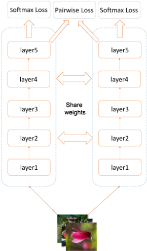
Considering this problem, we propose a pairwise loss between similar and dissimilar sample pairs to constrain the network for improving the classification performance.
Specifically, we construct a two-channel network with shared weights, and each network has its own softmax loss, which is shown in Figure 1. The proposed pairwise loss is added to one particular layer as a constraint of the learned feature representation. With this pairwise feature representation constraint, the classification performance can be improved. We will show that the contrastive loss used in the siamese network [Hadsell et al., 2006] is a special case of the proposed pairwise loss. The constraint of contrastive loss is too strong and thus may be unsuitable for real-world problems.
Pairwise constraints between samples are generally used to learn a distance metric. Distance metric learning has been applied to many machine learning problems, such as classification [Weinberger et al., 2006; Jin et al., 2009], clustering [Yeung and Chang, 2007], and retrieval [Hoi et al., 2010]. It aims to learn a transformation of the original feature, after which the distance between samples can be better estimated. However, the performance of distance metric learning is restricted due to the limitation of the feature representation and the ability of transformation. Considering its ability to learn high-level feature representations, deep learning has been used for distance metric learning. Hadsell et al. proposed a two-channel network (siamese network) with a contrastive loss for dimensionality reduction by learning an invariant mapping [Hadsell et al., 2006]. It relies solely on the neighborhood relationship to form the pairwise constraints. Considering the success of the siamese network, several works have followed this network architecture and also adopted the contrastive loss to address related problems. For example, Hyun et al. proposed a deep metric learning using lifted structured feature embedding [Oh Song et al., 2016]. Zagoruyko and Komodakis used a two-channel network to compare the similarity between image patches [Zagoruyko and Komodakis, 2015]. Sun et al. proposed a similar network architecture to learn face recognition neural networks [Sun et al., 2015]. This paper also reported that the loss of identification (classification) helped to improve the feature learning for verification. However, it did not discuss how the feature learning affected the classification performance. Similar to pairwise constraints, some deep metric learning methods use triplets as constraints to learn high-level feature representations [Cheng et al., 2016; Schroff et al., 2015; Hoffer and Ailon, 2015]. All these metric learning works focus on the neighborhood relationship and ignore the information directly provided by the class labels, which means that the procedure of composing similar or dissimilar pairs using labels may cause the loss of useful information. In this paper, we use the softmax loss to improve the performance of feature representation.
Overfitting is always a large issue in the training of deep architectures, particularly when the number of training samples is insufficient. Our proposed two-channel network can effectively prevent the overfitting problem and achieve promising results when the number of training samples is small. The reason is that the proposed pairwise loss can be viewed as a regularization of the network, which prevents the model from focusing on the label information too much. This will be demonstrated in the experiments.
The remainder of this paper is organized as follows. In Section 2, we present a detailed introduction to our proposed pairwise loss and the proposed two-channel joint learning network. Section 3 reports and analyzes various experimental results to demonstrate the effectiveness of our proposed method. Conclusions are presented in Section 4.
2 Classification and Representation Joint Learning
In this section, we provide a detailed introduction to our proposed joint learning of classification and representation. We first introduce the proposed pairwise loss and perform a comparison between our proposed pairwise loss and the commonly used contrastive loss. Then, the network architecture of combining classification and local distribution information is introduced. The stochastic gradient decent method is used to update the parameters of the network, and the updating algorithm is provided at the end of this section.
2.1 Proposed Pairwise Constraints
In this paper, the neighborhood relationships between sample pairs are used to obtain the local distribution information. Suppose that xi and xj are two input training samples in a d-dimensional feature space Rd . Yij indicates the similarity between xi and xj, and it is defined as
We can obtain the similarity between samples through class labels: two samples that have the same class label are similar, and two samples that have different class labels are dissimilar. Denote the square of the Euclidean distance between xi and xj on the output manifold as follows:
where f k (xi|θ) indicates the output of the network on the kth layer under parameters θ with input xi.
The main idea of the local distribution constraint is to learn a nonlinear mapping that maps similar input vectors to nearby points and dissimilar ones to distant points on the output manifold. Previous deep metric learning methods mainly used contrastive loss to achieve this goal. In this paper, we propose a pairwise loss that is motivated mainly by regularized distance metric learning [Jin et al., 2009]. Our proposed pairwise loss is more flexible than contrastive loss, which can be viewed as a special case of our pairwise loss. The explicit loss function can be formulated as follows:
where b and m are two parameters and 0 < b < m. Our proposed loss can guarantee that samples belonging to the same class are clustered and that the distance between dissimilar pairs is larger than the distance between similar pairs plus a margin. For a better understanding of the loss, it can be reformulated as follows:
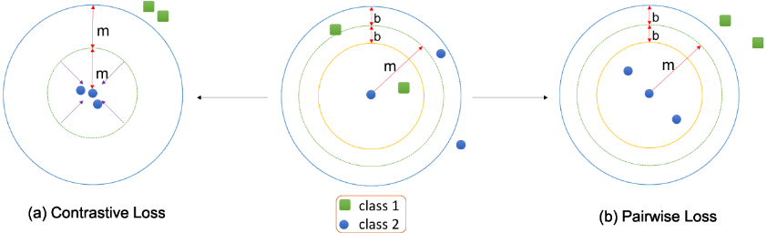
The contrastive loss of the siamese network can be viewed as a special case when setting the parameters of our pairwise loss as b = m and m = mc 2 , i.e.,
where mc is the margin of the contrastive loss function. The contrastive loss penalizes all similar pairs with a distance larger than zero. This constraint is too strong. It is more reasonable that the distance between similar pairs is a range within a margin rather than being zero. The comparison between our proposed pairwise loss and the contrastive loss is presented in Figure 2. In this figure, there are two classes of training samples, three blue circles and two green squares. In the original feature space, the distance between the samples in the same classes is larger than the distance between samples from different classes. After the training with our pairwise loss, the distance between similar pairs will be smaller than a margin m - b, and the distance between dissimilar pairs will be larger than m+ b. For contrastive loss, it is a special case of pairwise loss when b = m. In this case, the distance between similar pairs is constrained to be zero, which is too strong for real-world problems.
2.2 Network Architecture for Classification and Representation Joint Learning
To combine the information of class labels and the pairwise loss, we propose a two-channel network, as illustrated in Figure 1. This network has two types of loss functions: softmax loss on top of the network and pairwise loss constraints added to one particular layer. The softmax loss directly utilizes the information from the class labels, while the pairwise loss contributes to the local distribution. Note that the pairwise loss does not need to be added on top of the network. It can also be added on other layers. Suppose that we have a dataset χ that consists of N samples fromM different classes; the softmax loss can be formulated as follows:
where xi is the output of the network corresponding to training sample xi. 1{yi == t} is an indicator function. If yi == t is true (the class label of xi is t), then the result is 1; otherwise, the result is 0. ˆ pt is the predicted probability. W is the parameters of the softmax layer, and Wt is the weight of the t-th output, t = 1, · · · ,M.
By combing the softmax loss and the pairwise loss, the final optimization problem can be formulated as
where λ > 0 is one trade-off parameter. W1 and W2 are parameters of the two softmax losses. The two softmax losses have the same loss weight to guarantee the symmetry of the network. If only one softmax is added or the loss weights are different, then the two samples of the input pairs are treated unfairly, which may lead to a decrease in the performance. For softmax loss, the pairwise loss can be viewed as a regularization on the feature representation using local distribution information. It can be viewed as an indirect regularization on the parameters of the network. Consequently, it can prevent the network from overfitting. Furthermore, the local distribution information can also help improve the classification performance by providing more specific local distribution information. Additionally, it is slow and difficult for our proposed pairwise loss or contrastive loss to converge to a promising solution with random selection of training pairs. There are mainly two reasons. First, feeding all training pairs into the network requires too much time because of the large amount
Algorithm 1 Parameter updating algorithm of our proposed co-learning network
Input: Input data set χ = {(xi, yi)}Ni=1 , initializing the parameters of the network, learning rate ϵ, parameters b and m. Output: Parameters of the network.
- 1: while (not converge) do
- 2: Randomly select a pair of training samples (xi, yi) and (xj, yj).
- 3: ∇W1 = ∂CLoss(xi ,W1,yi) ∂W1
- 4: ∇W2 = ∂CLoss(xj ,W2,yj) ∂W2
- 5: ∇f k (xi|θk) = ∂PLoss(xi,xj,θ,k) ∂f k (xi|θk) + ∂CLoss(xi ,W1,yi) ∂f k (xi|θk)
- 7: ∇θk =∇f k (xi|θk) × ∂f k (xi|θk) ∂θk +∇f k (xj|θk) × ∂f k (xj|θk) ∂θk
- 8: Update W1 =W1 - ϵ∇W1, W2 =W2 - ϵ∇W2, θk = θk - ϵ∇θk.
- 9: end while
of possible pairs. Second, the learning rate used for the pairwise loss is generally small. However, the softmax loss does not have such drawbacks, which can help the pairwise loss converge faster and obtain a better solution. Consequently, the performance of feature representation can be improved.
We use the stochastic gradient decent method to update the parameters of the network. The learning algorithm is presented in Algorithm 1.
3 Experiments
To evaluate the effectiveness of our proposed method, we conduct various experiments on three benchmark datasets: MNIST, SVHN, and CIFAR10. All experiments are implemented using the CAFFE deep learning framework [Jia et al., 2014]. The first dataset used in our experiment is MNIST, which consists of a training set of 60000 28 × 28 handwritten digits of 10 classes and a test set of 10000 samples. The second dataset is the Street View House Numbers (SVHN), which consists of over 600000 32×32 color images of house number digits 0-9. This dataset is split into 73257 digits for training, 26032 digits for testing, and 531131 extra training digits that are less difficult to recognize. Note that the extra training digits are not used in any experiment in this paper. The third dataset used in our experiment is CIFAR10, which consists of 60000 32×32 color images from 10 classes. This dataset is split into 50000 training samples and 10000 test samples.
We compare our proposed method with several baselines. The first is the siamese network (siamese) with contrastive loss. The architecture of the siamese network is also a twochannel network but with only contrastive loss. The second is our pairwise loss (pairloss), which is supposed to have better performance than the siamese network. In the experiments, we randomly sample two batches of training samples into the two branches of the network and use the contrastive loss or pairwise loss on the top. The purpose of these two methods is to learn a high-level feature representation using pairwise constraints, and then a classifier (KNN or SVM) is applied on these features. The third method is to use softmax loss to improve the performance of pairwise loss (pair-soft). This will demonstrate that classification loss can derive better feature representation learning. The fourth method is the normal single-channel network with a softmax layer on the top to perform classification (singlenet). The final method is to combine the pairwise loss with softmax loss to improve the classification performance (pairnet), which will demonstrate that the local distribution information can provide more specific information than only using labels directly. The specific layer and parameter settings for each dataset are introduced in their own experiments.
3.1 MNIST Dataset
In this section, we present experimental details and the results on MNIST datasets. We use LeNet to conduct all experiments on MNIST. LeNet consists of 2 convolutional layers, and both of these layers are followed by a 2 × 2 max-pooling layers. Then, two fully connected layers are followed. The only preprocessing of the data is a global normalization that normalizes the pixel values of the image to 0-1. To train the models, we randomly select different numbers (60, 100, 500, and 1000 samples for each class) of training samples from the training set. We also train the model by using all training samples in the training set (denoted as "ALL"). All random selections are repeated three times to avoid randomness. A KNN classifier is applied on the learned features via contrastive loss, pairwise loss and pair-soft loss. The experimental results are summarized in Table 1.
From the results in Table 1, we can conclude that our pairwise loss outperforms the contrastive loss with different amounts of training samples. Comparing the results between pairloss and pair-soft, it is clear that the softmax loss helps to improve the performance of the pairwise loss, which means that a better feature representation is learned. The pairnet performs considerably better than singlenet, particularly when the number of training samples is small, which demonstrates the effectiveness of the combination of pairwise loss and softmax loss. When the number of training samples is small, the information provided directly by the class label is limited. However, the pairwise constraints can provide more information about the feature distribution, leading to better classification performance.
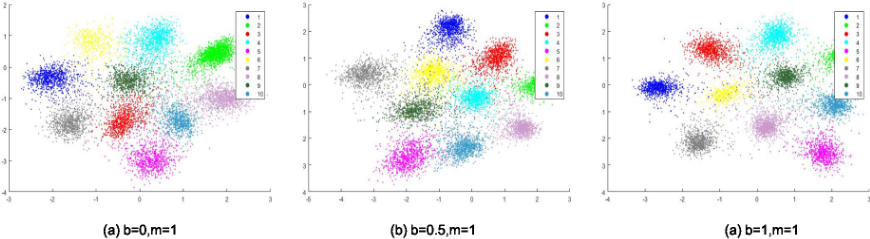
We conduct another experiment to verify the feature representation learning ability of our proposed pairwise loss and analyze the effects of the parameters by visualizing the features in 2-D space. We add another fully connected layer on top of the network and set the output dimensionality as 2. The pairwise loss is used to learn feature representations by setting the parameter b to 0, 0.5, and 1. The final results are shown in Figure 3. Each of the sub-figures has 10 clusters corresponding to digits 0-9. In the illustration of Figure 2, we can observe that when the parameter b is set to smaller values, the circle that constrains the similar pairs will be larger. This result means that the size of the clusters is larger. From the results presented in Figure 3, we can observe that the size of the cluster decreases with the value of parameter b varying from 0-1. When the value of b is set to 1, which is equal to parameter m, this can be viewed as contrastive loss used in the siamese network.
| Methods | ALL | 10000 | 5000 | 1000 | 600 |
|---|---|---|---|---|---|
| siamese | 0.9731 | 0.9715± 0.0017 | 0.9674 ± 0.0026 | 0.9379 ± 0.0054 | 0.9171 ± 0.0029 |
| pairloss | 0.9795 | 0.9791± 0.0003 | 0.9753 ± 0.0022 | 0.9432 ± 0.0062 | 0.9257 ± 0.0043 |
| pair-soft | 0.9908 | 0.9864± 0.0007 | 0.9824 ± 0.0008 | 0.9630± 0.0044 | 0.9517±0.0037 |
| singlenet | 0.9892 | 0.9820± 0.0022 | 0.9739 ± 0.0029 | 0.9397 ± 0.0064 | 0.9247 ± 0.0116 |
| pairnet | 0.9917 | 0.9875±0.0007 | 0.9834±0.0001 | 0.9637±0.0019 | 0.9510±0.0057 |
3.2 SVHNDataset
In this section, we conduct experiments on the SVHN dataset. The network architecture used for the SVHN dataset consists of 3 convolutional layers, and each of them is followed by a max-pooling layer. ReLU non-linearity is applied between two convolutional layers. Two fully connected layers are added after the convolutional layers. Note that the extra training dataset is not used in our experiments. We preprocess the images using local contrast normalization [Zeiler and Fergus, 2013] due to the large variety of colors and brightness variations in the images. After the local contrast normalization, we crop the image into a 28 × 28 patch that is located in the center of the image. No data augmentation is applied in our experiments. To train the models, we randomly select different numbers (2000 and 500 samples for each class) of training samples from the training set. We also train the model by using all training samples in the training set (denoted as
| Methods | ALL | 20000 | 5000 |
|---|---|---|---|
| siamese | 0.8886 | 0.8730 ± 0.0010 | 0.7887 ± 0.0109 |
| pairloss | 0.8998 | 0.8779 ± 0.0038 | 0.8112 ± 0.0172 |
| pair-soft | 0.9080 | 0.8934 ± 0.0009 | 0.8552 ± 0.0010 |
| singlenet | 0.9219 | 0.8855 ± 0.0006 | 0.8426 ± 0.0081 |
| pairnet | 0.9387 | 0.9171±0.0014 | 0.8876±0.0010 |
| Methods | ALL | 10000 | 5000 |
|---|---|---|---|
| siamese-soft | 0.805 | 0.7286 ± 0.0145 | 0.6677 ± 0.0338 |
| pair-soft | 0.8259 | 0.7430 ± 0.0075 | 0.6789 ± 0.0254 |
| singlenet | 0.8374 | 0.7357 ± 0.0022 | 0.6671 ± 0.0095 |
| pairnet | 0.8609 | 0.7612±0.0107 | 0.7055±0.0002 |
"ALL"). All random procedures are repeated three times, and the average performance is reported to avoid randomness. A KNN classifier is applied on the learned features. The results are shown in Table 2.
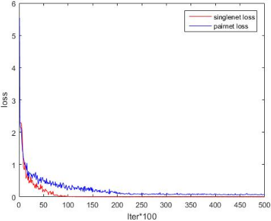
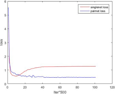
From Table 2, we can obtain conclusions similar to those from the experiments on the MNIST dataset. The pairwise loss and the softmax loss help to improve the performance of each other consistently. The improvement is particularly obvious when the amount of training samples is small. Additionally, we present results to demonstrate the ability of our proposed method to prevent overfitting in Figure 4 and Figure 5. We randomly select 500 samples from each class and use the same network as used in the above experiments on SVHN. We compare the proposed pairnet with singlenet to verify its ability to prevent overfitting. Note that the same weight decay is used for these two networks. From Figure 4 and Figure 5, we can conclude that the training loss of singlenet decreases quickly to a value of approximately zero. However, the test loss of singlenet increases after a certain training iteration, which means an overfitting training process. Our pairnet can effectively prevent the overfitting problem with the regularization via pairwise loss on the feature representation.
3.3 CIFAR10 Dataset
We also conduct experiments on the CIFAR10 dataset. This dataset is more difficult than the MNIST dataset and the SVHN dataset. Consequently, the architecture of the network used for training CIFAR10 is more complex. We adopt a network similar to that used in [Hoffer and Ailon, 2015], which consists of 4 convolutional layers and 1 fully connected layer. Each of the first three convolutional layers is followed by a max-pooling layer. A ReLU layer is applied between two consecutive layers. Finally, a softmax layer is added on the top of the network for classification. The images are preprocessed by performing global contrast normalization as used for the SVHN dataset. Then, ZCA whitening is performed, which makes the pixels less correlated with each other and have the same variances [Srivastava et al., 2014]. Note that the training of the network converges slowly if we use only contrastive loss or pairwise loss, which mainly has two reasons. First, CIFAR10 is more difficult, and the network architecture is more complicated. Second, the number of pairs in our model in each batch is small due to the storage limitations of the GPU. Consequently, we do not compare the performance of contrastive loss and pairwise loss. Rather, we add a softmax loss on top of the siamese network (siamesesoft) and compare its performance with the other methods. We first compare the performance using all the training data and then randomly select 1000 and 500 samples from each class as the training set to compare the performance of all the methods. Each random selection is repeated three times to avoid randomness. The results are shown in Table 3.
Note that SVM is used to classify the learned features of siamese-soft and pair-soft. From the results presented in Table 3, we can conclude that our proposed pairnet outperforms the other methods. The contrastive loss and pairwise loss converge faster through training with a softmax loss, and both of the methods can obtain performance comparable to that of singlenet.
4 Conclusions
In this paper, we propose a deep network architecture to learn classification and feature representation simultaneously, which can enhance the performance of each other. A pairwise loss is proposed to constrain the feature representation learning. Then, we propose a two-channel network with the proposed pairwise loss as a regularization of the feature distribution. The classification performance can be improved with this regularization. Additionally, the softmax loss used in classification can also help to learn better feature representations. The pairwise loss can be viewed as an indirect regularization on the weights of the network, which prevents overfitting when the training samples are insufficient. Extensive experiments are conducted on three benchmark datasets, and the experimental results demonstrate the effectiveness of our proposed method.
Acknowledgments
This work was supported in part by the 973 Project 2015CB351803; in part by NSFC projects 61572451, 61390514 and 61632019; in part by the Youth Innovation Promotion Association CAS under Grant CX2100060016; in part by the Fok Ying Tung Education Foundation under Grant WF2100060004; and in part by the Australian Research Council Projects FT-130101457, DP-140102164, and LP-150100671.
@inproceedings{ijcai2017p308,
  title     = {Classification and Representation Joint Learning via Deep Networks},
  author    = {Li, Ya and Tian, Xinmei and Shen, Xu and Tao, Dacheng},
  booktitle = {Proceedings of the Twenty-Sixth International Joint Conference on
               Artificial Intelligence, {IJCAI-17}},
  publisher = {International Joint Conferences on Artificial Intelligence Organization},
  editor    = {Carles Sierra},
  pages     = {2215--2221},
  year      = {2017},
  month     = {8},
  note      = {Main track},
  doi       = {10.24963/ijcai.2017/308},
  url       = {https://doi.org/10.24963/ijcai.2017/308},
}
TY - CPAPER TI - Classification and Representation Joint Learning via Deep Networks AU - Li, Ya AU - Tian, Xinmei AU - Shen, Xu AU - Tao, Dacheng T2 - Proceedings of the Twenty-Sixth International Joint Conference on Artificial Intelligence, IJCAI-17 PB - International Joint Conferences on Artificial Intelligence Organization PY - 2017 SP - 2215 EP - 2221 DO - 10.24963/ijcai.2017/308 UR - https://doi.org/10.24963/ijcai.2017/308 ER -Copied
Machine-readable versions of this paper, for tools and AI agents:





