
Fast Recursive Low-rank Tensor Learning for Regression
Proceedings of the Twenty-Sixth International Joint Conference on Artificial Intelligence. Main track. Pages 1851-1857.
https://doi.org/10.24963/ijcai.2017/257
Keywords
- Machine Learning: Online Learning
- Machine Learning: Structured Learning
- Machine Learning: Time-series/Data Streams
- Machine Learning: Machine Learning
Abstract
In this work, we develop a fast sequential low-rank tensor regression framework, namely recursive higher-order partial least squares (RHOPLS). It addresses the great challenges posed by the limited storage space and fast processing time required by dynamic environments when dealing with large-scale high-speed general tensor sequences. Smartly integrating a low-rank modification strategy of Tucker into a PLS-based framework, we efficiently update the regression coefficients by effectively merging the new data into the previous low-rank approximation of the model at a small-scale factor (feature) level instead of the large raw data (observation) level. Unlike batch models, which require accessing the entire data, RHOPLS conducts a blockwise recursive calculation scheme and thus only a small set of factors is needed to be stored. Our approach is orders of magnitude faster than all other methods while maintaining a highly comparable predictability with the cutting-edge batch methods, as verified on challenging real-life tasks.
- [Bahadori et al., 2014] Mohammad Taha Bahadori, Qi Rose Yu, and Yan Liu. Fast multivariate spatio-temporal anal- ysis via low rank tensor learning. In Advance in Neural Information Processing Systems, pages 3491-3499, 2014.
- [Bro, 1996] Rasmus Bro. Multiway calidration. multilinear PLS. Journal of Chemometrics, 10:47-61, 1996.
- [Chao et al., 2010] Zenas C Chao, Yasuo Nagasaka, and Naotaka Fujii. Long-term asynchronous decoding of ar- m motion using electrocorticographic signals in monkeys. Frontiers in Neuroengineering, 3, 2010.
- [Cichocki et al., 2009] Andrzej Cichocki, Rafal Zdunek, Anh Huy Phan, and Shun-ichi Amari. Nonnegative ma- trix and tensor factorizations: applications to exploratory multi-way data analysis and blind source separation. John Wiley and Sons, 2009.
- [De Lathauwer et al., 2000a] Lieven De Lathauwer, Bart De Moor, and Joos Vandewalle. A multilinear singular value decomposition. SIAM Journal on Matrix Analysis and Applications, 21(4):1253-1278, 2000.
- [De Lathauwer et al., 2000b] Lieven De Lathauwer, Bart De Moor, and Joos Vandewalle. On the best rank-1 and rank-(r 1, r 2,..., rn) approximation of higher-order ten- sors. SIAM Journal on Matrix Analysis and Applications, 21(4):1324-1342, 2000.
- [Eliseyev and Aksenova, 2013] Andrey Eliseyev and Tetiana Aksenova. Recursive n-way partial least squares for brain- computer interface. PloS One, 8(7):e69962, 2013.
- [Harshman, 1970] Richard A Harshman. Foundations of the parafac procedure: Models and conditions for an" explana- tory" multi-modal factor analysis. 1970.
- [Hou and Chaib-draa, 2016] Ming Hou and Brahim Chaib- draa. Online incremental higher-order partial least squares regression for fast reconstruction of motion trajectories from tensor streams. In International Conference on A- coustics, Speech, and Signal Processing. IEEE, 2016.
- [Kim et al., 2005] Hyunsoo Kim, Jeff X Zhou, Herbert C Morse III, and Haesun Park. A three-stage framework for gene expression data analysis by L1-norm support vector regression. International Journal of Bioinformatics Re- search and Applications, 1(1):51-62, 2005.
- [Luo et al., 2015] Lijia Luo, Shiyi Bao, and Zengliang Gao. Quality prediction based on hopls-cp for batch process- es. Chemometrics and Intelligent Laboratory Systems, 143:28-39, 2015.
- [O'Hara, 2010] Michael J O'Hara. On low-rank updates to the singular value and tucker decompositions. In SIAM International Conference on Data Mining, pages 713-719.
- [Sun et al., 2008] Jimeng Sun, Dacheng Tao, Spiros Pa- padimitriou, Philip S Yu, and Christos Faloutsos. Incre- mental tensor analysis: Theory and applications. Transac- tions on Knowledge Discovery from Data, 2(3):11, 2008.
- [Van Der Aa et al., 2011] NP Van Der Aa, X Luo, GJ Gieze- man, RT Tan, and RC Veltkamp. Utrecht multi-person motion (UMPM) benchmark. Technical report, Citeseer, 2011.
- [Yu et al., 2015] Rose Yu, Dehua Cheng, and Yan Liu. Ac- celerated online low-rank tensor learning for multivariate spatio-temporal streams. In International Conference on Machine Learning, pages 238-247, 2015.
- [Zhao et al., 2011] Qibin Zhao, Cesar F Caiafa, Danilo P Mandic, Liqing Zhang, Tonio Ball, Andreas Schulze- Bonhage, and Andrzej Cichocki. Multilinear subspace re- gression: An orthogonal tensor decomposition approach. In Advance in Neural Information Processing Systems, volume 2011, pages 1269-1277, 2011.
- [Zhao et al., 2013] Qibin Zhao, Cesar F Caiafa, Danilo P Mandic, Zenas C Chao, Yasuo Nagasaka, Naotaka Fujii, Liqing Zhang, and Andrzej Cichocki. Higher order partial least squares (HOPLS): a generalized multilinear regres- sion method. IEEE Transactions on Pattern Analysis and Machine Intelligence, 35(7):1660-1673, 2013.
- [Zhao et al., 2014] Qibin Zhao, Guoxu Zhou, Liqing Zhang, and Andrzej Cichocki. Tensor-variate gaussian processes regression and its application to video surveillance. In In- ternational Conference on Acoustics, Speech, and Signal Processing, pages 1265-1269. IEEE, 2014.
- [Zhou et al., 2013] Hua Zhou, Lexin Li, and Hongtu Zhu. Tensor regression with applications in neuroimaging data analysis. Journal of the American Statistical Association, 108(502):540-552, 2013.
References were extracted automatically from the PDF and may contain errors.
Full text extracted automatically from the PDF; figures, tables and equations may differ. The PDF is the version of record.
1 Introduction
Tensor-variate regression approaches arise frequently in the machine learning community because of the increasing demands to deal with the problems that usually involve largescale higher-order data with complex structures. Such problems abound in a broad range of applications, including computer vision [Zhao et al., 2014], neural signal processing [Zhao et al., 2011; 2013; Eliseyev and Aksenova, 2013], medical imaging data analysis [Zhou et al., 2013], climate data analysis [Bahadori et al., 2014], and are in general very challenging to solve. One of these approaches in widespread use is N-way partial least squares (NPLS) [Bro, 1996] which carries out a joint CP (CANDECOMP/PARAFAC) decomposition [Harshman, 1970] of tensorial input and output into sum of rank-one tensors. To overcome the low predictability and the slow convergence rate of NPLS, the state-of-theart higher-order partial least squares (HOPLS) [Zhao et al., 2011; 2013] has been proposed based on the joint orthogonal block Tucker decomposition [De Lathauwer et al., 2000a] of input and output tensors. The most preferable property of HOPLS over NPLS lies in its power to provide superior predictability with optimal balance between fitness and model complexity [Zhao et al., 2013].
For many real-world applications, however, high-order big size tensorial data often take the form of extremely large or even infinite tensor sequences, especially in time-critical dynamic environments, where the new data keep coming fast over time. Although we can apply the batch method to all the data each time a new pair arrives, in this case HOPLS can quickly become computationally prohibitive or merely infeasible. Moreover, it is often impossible to store the whole data or require them to be available up front. Thus, the memory efficient sequential methods are absolutely essential.
Among the methods that can recursively handle the data, the recursive N-way partial least squares (RNPLS) [Eliseyev and Aksenova, 2013] processes the tensor sequences by unifying a recursive calculation scheme with the multiway data representation of NPLS. Inheriting the drawbacks of NPLS, RNPLS likewise suffers from the lack of adequate accuracy and the slow convergence rate because of its CP-based solution. Thus, the speed is rather slow especially when a relatively larger number of latent vectors are required for sufficient accuracy, significantly reducing the applicability of RNPLS in many time-critical applications [Zhao et al., 2013]. Another recent work named accelerated low-rank tensor online learning (ALTO) [Yu et al., 2015] has been proposed for the speed of processing spatio-temporal tensor sequence using a random low-rank projection technique. However, ALTO is only restricted to spatio-temporal data structure which demands the input and output tensors are at least in common on structures along the spatial and temporal modes.
In this paper, we introduce a super-fast tensor regression framework, called recursive higher-order partial least squares (RHOPLS), for sequential blockwise processing of general tensor sequences. Our contributions are: (i) designing a recursive framework that efficiently updates the regression coefficients (factors) at a small-scale factor (feature) level instead of the large raw data (observation) level by integrating a low-rank modification strategy of the Tucker [O'Hara, 2010] into PLS; (ii) developing an efficient algorithm based on a series of computationally advantageous calculations yet with only a small number of factors for storage; (iii) applying RHOPLS to several challenging tasks such as estimation of human pose from videos, showing the great potentiality for fast real-time predictions of human pose positions. In brief, our framework does not suffer from neither inferior predictability nor poor convergence rate of NPLS-based models. It is also free from the computational issues related to the HOPLS-based models when the data order, "sample" or "dimensionality" complexity is high. Finally, our RHOPLS exhibits highly competitive accuracy with the best batch methods but is extremely faster than other sequential methods.
2 Recursive Higher-order PLS
2.1 Preliminaries and Problem Setting
Throughout the paper, higher-order tensors will be denoted as X ∈ RI1×I2×···×ID in calligraphy letters, where D is the order of X. The d-mode unfolding of X, defined as X(d) ∈ RId×I1···Id-1Id+1···ID , is the process of rearranging the d-mode vectors into the columns of the resulting matrix. We refer to d-mode product of tensor X ∈ RI1×I2×···×ID and matrix A ∈ RJd×Id as Y = X ×d A ∈ RI1×···×Id-1×Jd×Id+1×···×ID . We use contracted product of tensors X ∈ RI1×···×IC×J1×···×JP and Z ∈ RI1×···×IC×K1×···×KQ along the same C modes to define the cross-covariance tensor [Zhao et al., 2013] Y as
The Tucker decomposition can be expressed as Y ≈ G ×1 A(1) ×2 · · ·×D A(D) , where A(d) ∈ RId×Rd is the factor matrix. G ∈ RR1×R2×···×RD represents the core tensor indicating the interaction among factor matrices in different modes. Rd serves as the d-rank of Y in mode d.
Without the loss of generality, we consider an Nth-order input tensor X ∈ RI1×···×IN and anMth-order output tensor Y ∈ RJ1×···×JM with coupled observations, namely I1 = J1 and we process the data in terms of mini-batch of size b, say {X (t) ∈ Rb×I2×···×IN , Y(t) ∈ Rb×J2×···×JM } for minibatch t. I0 will stand for the number of initial observations. We use I to denote the maximum index of all modes, while R is the maximum d-rank of all modes which are supposed to be small in practice, i.e., R≪ I. Finally, F is the number of latent vectors, while L and K are used to denote the collection of d-ranks for the input and output loadings, respectively.
2.2 General Framework
As mentioned in Section 1, sequential approaches to regression are capable of handling big data as well as online data. In this context, the key idea behind RNPLS [Eliseyev and Aksenova, 2013] is to directly add the old tensor data, represented by refolding the previous set of factors into a fixed data size, to the new arriving tensor data to generate the joint tensor data, and then applies NPLS to joint tensor data to estimate the new set of factors. Although recursively handling the new data, RNPLS has one major disadvantage in that it has to perform a slow iterative NIPALS-style procedure on the joint tensor data at the level of original dimensionality I. Furthermore, RNPLS represents the old tensor via a refolding operation of the factor matrices into tensor, which may cause undesired errors of approximating the old tensor data.
Different from RNPLS, we propose to recursively merge the new data into the old one in terms of the factors rather than considering the raw tensor data. Our framework directly updates the PLS-related parameters at much smaller scale using a closed-form solution, thus inexpensively keeping track of the subspace patterns and the summary of model status.
Generally speaking, up to the point t - 1, the set of old factors representing the model summarizes the total variation in all previous mini-batches, and hence approximates the current modeling state. Then, a newly arriving mini-batch t is decomposed into a set of incremental factors which contain the variation merely corresponding to the new data. Our framework carries out a recursive update procedure that effectively yet inexpensively "absorbs" the incremental factors into the old ones to produce a set of new factors at t. Continuing in the same spirit, we are able to efficiently process the new data in a mini-batch way over time. Figure 1 illustrates the whole scheme that consists of the following principal steps as below. We choose N = 3 order input tensor and M = 2 order output tensor for simplicity of visualization.
In what follows, Step 0 is a preprocessing step that executes only once, while the other steps are conducted repeatedly for each new mini-batch. With the extracted loadings and individual core tensors in hand, the PLS-based regression coefficients can be formed in terms of these extracted factors and the prediction can be made similar to the one in HOPLS [Zhao et al., 2013].
Step 0: Initial Approximation (red arrow)
As for the initial tensor pair {X(0) ∈ RI0×I2×···×IN , Y(0) ∈ RI0×J2×···×JM }, we aim to extract a set of initial factors. Instead of using a deflation process of block tensor terms in HOPLS [Zhao et al., 2011; 2013], we simply apply the standard Tucker to jointly decompose the initial data pair such that the latent components extracted from X(0) and Y(0) have the maximum pairwise covariance, which is of the form
where G x (0) ∈ RL1×L2×···×LN and G y (0) ∈ RK1×K2×···×KM serve as core tensors with L1 = K1. T(0) ∈ RI0×L1 is the common latent matrix, while {P(n) (0)}Nn=2 ∈ RIn×Ln and {Q(m) (0)}Mm=2 ∈ RJm×Km are the loadings corresponding to X(0) and Y(0), respectively. To solve above factors, we first form the 1-mode cross-covariance tensor C(0) =< X(0), Y(0) >{1:1} which follows by estimating the loadings using a higher-order orthogonal iteration (HOOI) [De Lathauwer et al., 2000b]
Here, G xy (0) ∈ RK2×···×KM×L2×···×LN is said to be 1-mode cross-covariance core tensor. Having obtained all the loadings, the core tensors and common latent matrix can be calculated according to (1) and (2) using higher-order singular vector decomposition (HOSVD) [De Lathauwer et al., 2000a].
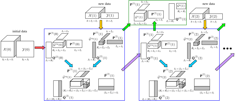
These factors (common latent matrix, loadings, core tensors and the 1-mode cross-covariance core tensor), indicating the initial modeling state, are to be updated on new mini-batch.
Step 1: Incremental Approximation (yellow arrow)
Turning to mini-batch t, a new tensor pair {X(t) ∈ Rb×I2×···×IN , Y(t) ∈ Rb×J2×···×JM } with small size b comes into the picture. To approximate the incremental data efficiently, we propose to collect the set of factors by first performing partial Tucker to X(t) and Y(t) separately, such that all the modes except the first mode are decomposed with d-ranks rank-(¯L2, ..., ¯LN) and rank-( ¯K2, ..., ¯KM)
Thereafter, the 1-mode cross-covariance core tensor ¯ G xy (t) is immediately formed exploiting only the core tensors ˇ G x (t) and ˇ G y (t) as ¯ G xy (t) =< ˇ G x (t), ˇ G y (t) >{1:1}, where ¯ G xy (t) ∈ R ¯K2×···× ¯KMׯL2×···×¯LN can be calculated using only O(RM+N-2 ). In total, the cost for approximating the incremental data requires merely O(max(RM+N-2 , RI M-1 , RI N-1 )). Note that the HOPLS has to compute and decompose the 1-mode cross-covariance tensor of size J2 × · · · × JM × I2 × · · · × IN using entire data when estimating each one of R latent vectors [Zhao et al., 2013], leading to total cost as large as O(RI M+N-1 ). In HOPLS, calculating and decomposing such huge tensor R times yields substantial costs especially when data dimensionality, data order and d-ranks are large. In contrast to HOPLS, our Step 1 overcomes this drawback by first partially decomposing only the new mini-batch input and output individually via Tucker and then calculating the desired cross-covariance core tensor to gather the incremental factors. This step contributes to the speed-ups mainly from the perspective of significantly reducing the "dimensionality" complexity, because we extract eigenvectors on two much smaller-scale individual minibatch tensors instead of on a massive cross-covariance tensor, and we also form the cross-covariance core tensor at the core tensor scale of R instead of at the original dimensionality I.
Step 2: Expansion (blue arrow)
Inspired by the work [O'Hara, 2010], we first append the set of incremental factors associated with the new mini-batch to the set of old factors that corresponds to the current model status, resulting in an augmented set of factors. Unlike [O'Hara, 2010], we apply this strategy to the cross-covariance core tensor in a PLS framework involving both input-output tensors rather than just single tensor as in [O'Hara, 2010]. Specifically, concatenating the variation captured by loading ¯P(n) (t) ∈ RInׯLn to P(n) (t - 1) ∈ RIn×Ln , we can get the augmented variation via loading ˆP(n) (t) = [P(n) (t - 1) ¯P(n) (t)] ∈ RIn×(Ln+¯Ln) , where n = 2, ...,N. Likewise, we obtain the loading ˆQ(m) (t) = [Q(m) (t - 1) ¯Q(m) (t)] ∈ RJm×(Km+ ¯Km) for m = 2, ...,M. We can also get the augmented 1-mode cross-covariance core tensor ˆ G xy (t) ∈ R(K2+ ¯K2)×···×(KM+ ¯KM)×(L2+¯L2)×···×(LN+¯LN) by appending ¯ G xy (t) ∈ R ¯K2×···× ¯KMׯL2×···×¯LN to G xy (t - 1) ∈ RK2×···×KM×L2×···×LN in a super block-diagonal manner, leaving other new entries to be zeros.
Step 3: Compression (purple arrow)
We next truncate the set of augmented factors back into the set of factors with the size of original d-ranks, which means finding the most dominant principal components in the subspaces of loadings out of the augmented set of loadings. To this end, the augmented factors {ˆP(n) (t)}Nn=2 , {ˆQ(m) (t)}Mm=2 and ˆ G xy (t) described in last step are truncated to produce new loadings {P(n) (t)}Nn=2 ∈ RIn×Ln , {Q(m) (t)}Mm=2 ∈ RJm×Km as well as 1-mode cross-covariance core tensor G xy (t) ∈ RK2×···×KM×L2×···×LN , hence keeping track of the change of patterns in each loading subspace, leading to
- compute QR factorization on the augmented loadings ˆP(n) (t) = Ux(n)Vx(n) , where Ux(n) ∈ RIn×(Ln+¯Ln) and Vx(n) ∈ R(Ln+¯Ln)×(Ln+¯Ln) for n = 2, ...,N; ˆQ(m) (t) = Uy(m)Vy(m) , Uy(m) ∈ RJm×(Km+ ¯Km) and Vy(m) ∈ R(Km+ ¯Km)×(Km+ ¯Km) for m = 2, ...,M.
- transform cross-covariance core tensor ˆ G xy (t) to get
- calculate the rank-(L2, ...,LN,K2, ...,KM) orthogonal Tucker on the core ˜ G xy (t) to get the resulting 1-mode cross-covariance core tensor G xy (t) for mini-batch t
The purpose of above operations is to maintain computations at small cross-covariance core tensor level of R instead of at huge cross-covariance tensor level of I, the dominating cost is thus reduced to O(RN+M-1 ) fromO(I N+M-1 ). In a word, Steps 2 and 3 together are applied to 1-mode cross-covariance core tensor for purpose of updating the loading factors, which contributes in part to the speed-ups from perspective of reducing the "sample" complexity to a low constant level.
Step 4: Projection (green arrow)
Finally, we propose to update the individual core tensors of input and output from the internal representation of model under the projection of loadings obtained in the last step. These individual core tensors in conjunction with loadings are exploited to produce the final prediction. Specifically, we begin with reconstruction of the old internal tensor representation Xint(t-1) ∈ RI0×L2×···×LN from the latent matrix T(t-1), the loadings {P(n) (t - 1)}Nn=2 and the core tensor G x (t - 1) under the projection of current loadings {P(n) (t)}Nn=2 as
Meanwhile, we also reconstruct the incremental internal tensor representation ¯ Xint(t) ∈ Rb×L2×···×LN from the core tensor ˇ G x (t) and loadings {¯P(n) (t)}Nn=2 obtained in Step 1 by projecting onto the subspaces of the current loadings {P(n) (t)}Nn=2 , which becomes
After concatenating ¯ Xint(t) to Xint(t - 1), we get Xint(t) ∈ R(I0+b)×L2×···×LN as the augmented internal representation. Then, Xint(t) is decomposed using Tucker-1 model [Cichocki et al., 2009] to get the common internal latent matrix Tint(t) ∈ R(I0+b)×L1 and core G x (t) ∈ RL1×L2×···×LN as
where Tint(t) is thereafter truncated to keep the very last I0 rows, leading to the common T(t) ∈ RI0×L1 for the purpose of internal representation reconstruction of the model in the subsequent mini-batch. Similarly, we finally have Yint(t) ∈ R(I0+b)×K2×···×KM and G y (t) ∈ RK1×K2×···×KM for the output side. By employing our proposed projection strategy, the dominating cost of this step is substantially cut down from O(max(I0I N , I N+1 )) to O(max(I0RN ,RN+1 )), because we equivalently represent the model and calculate the new factors in terms of projected internal tensors that lie in the tensor space with small scale R but large original I. Step 4 is responsible for efficiently updating the individual core tensors, which also contributes in part to the total acceleration by reducing the "sample" complexity.
Note that RHOPLS demands a minimum space complexity in the sense that only a small number of factors, dominating by O(max(RN+M-2 )) of cross-covariance core tensor, are needed to be stored to represent the running model.
2.3 RelatedWork
In contrast to the standard (batch) Tucker, incremental tensor analysis (ITA) [Sun et al., 2008] has been proposed as an incremental tensor approximation tool that dynamically updates a Tucker approximation using new arriving data. However, ITA is a component model that is restricted to unsupervised learning settings only, focusing only on a single tensor rather than input-output tensor pairs in supervised regression settings. As an another incremental tensor approximation tool, incremental Tucker (IT) [O'Hara, 2010] additively updates the Tucker model using a low-rank subspace truncation strategy. Like ITA, IT is a component model that considers single tensor in the context of unsupervised learning only and cannot be directly applied to the tensor regression tasks. Our Step 2 and 3 are adapted from the basic idea of this tool, however, we here propose to integrate IT as just one part of our whole PLS-based framework to extract loadings. Notice that the major contribution of our RHOPLS is from the system level, all the steps are essential to the whole framework and should not be treated separately. Moreover, we like to stress that the concepts of tensor decomposition tool, i.e., Tucker, ITA or IT, are fundamentally different from tensor regression models w.r.t. the targeted goal, algorithm and applications.
3 Experimental Results
In our experiments, the root mean squares of prediction (RMSEP) [Kim et al., 2005] as well as the Q index [Luo et al., 2015] are used to quantitatively gauge the predictive performance of our approach. We recorded the CPU learning time per new mini-batch for all recursive methods, and we also gave CPU learning time for batch methods using the entire training set. We compared RHOPLS with NPLS [Bro, 1996], RNPLS [Eliseyev and Aksenova, 2013], HOPLS [Zhao et al., 2013] and IHOPLS [Hou and Chaib-draa, 2016] on general tensorial sequences with no special structures assumed in contrast to spatio-temporal data. To show the robustness, each sequence was randomly shuffled into 10 instances for evaluation, because our framework is designed for the general setting of sequence though it could be applied to the infinite stream. One half of the shuffled sequence served as training set while the remaining half was used for test. The optimal hyper-parameters of all methods were determined by crossvalidation, so that their best performance could be exhibited balancing between speed and accuracy. In particular, the convergence criterion and the maximum iterations of RNPLS for were selected to 10-5 and 40. For RHOPLS, the initial number of latent vectors F and initial input loadings L and output loadings K are needed to be tuned, so are the incremental loadings ∆L and ∆K. For simplicity, we assumed L = ∆L and K = ∆K just to reduce the number of hyper-parameters, and L, K are tuned by conducting a grid search on the combination of typical values, i.e., for L of a 3rd-order input tensor, we might search on [4, 8], [8,12], [12,16], [16,20] ... and so on. All tests were done on a server of 12 cores 3.20GHz CPU.
| UMPM 24 × 32 | Scenario "triangle" X ∈ R1230×24×32 | Scenario "table" X ∈ R1430×24×32 | |||||
|---|---|---|---|---|---|---|---|
| Methods | Hyper-parameters | Q | RMSEP | Time (s) | Q | RMSEP | Time (s) |
| NPLS | F = 25(triangle), 30(table) | .8431 (.0070) | 132.0 (6.3) | 16.0 (2.6) | .8240 (.0067) | 151.2 (6.0) | 25.4 (2.7) |
| RNPLS | F = 25(triangle), 30(table), γ = 1 | .8011 (.0092) | 169.4 (8.7) | 6.17 (1.25) | .7865 (.0083) | 184.7 (7.1) | 8.06 (1.47) |
| HOPLS | F = 40, L = [8, 12], K = [3, 9] | .8480 (.0019) | 127.8 (2.2) | 6.47 (0.34) | .8388 (.0045) | 139.1 (3.8) | 6.94 (0.38) |
| F = 40, L = [12, 16], K = [3, 9] | .8462 (.0016) | 129.0 (2.3) | 5.94 (0.22) | .8341 (.0058) | 142.7 (4.8) | 6.04 (0.80) | |
| IHOPLS | F = 40,L = [12, 16], K = [3, 9] | .7034 (.0104) | 248.5 (8.8) | 4.48 (0.45) | .7393 (.0069) | 227.2 (8.1) | 4.53 (0.42) |
| RHOPLS | F = 40,L = [8, 12], K = [3, 9] | .8453 (.0035) | 129.6 (2.8) | 0.25 (0.01) | .8304 (.0058) | 145.3 (5.7) | 0.24 (0.01) |
| F = 40, L = [12, 16], K = [3, 9] | .8430 (.0039) | 132.3 (3.0) | 0.26 (0.01) | .8294 (.0072) | 146.8 (6.0) | 0.25 (0.01) | |
| UMPM240 × 320 | Scenario "triangle" | Scenario "table" | ||
|---|---|---|---|---|
| Methods | Q | Time (s) | Q | Time (s) |
| NPLS | .8604 | 540.8 | .8454 | 849.7 |
| RNPLS | .8105 | 39.9 | .7997 | 58.3 |
| HOPLS | .8774 | 53.0 | .8670 | 57.8 |
| .8801 | 56.1 | .8709 | 59.1 | |
| IHOPLS | .7115 | 26.3 | .7519 | 27.4 |
| RHOPLS | .8722 | 0.26 | .8524 | 0.27 |
| .8786 | 0.28 | .8602 | 0.30 | |
3.1 Utrecht Multi-PersonMotion Database
We first tested RHOPLS on the Utrecht Multi-Person Motion (UMPM) benchmark [Van Der Aa et al., 2011], which provides the simultaneous recordings of video sequences and 3D ground truth positions of human natural motions in daily life activities. For our test, the input data was an intensity image sequence from the front camera at 25fps, taking the form of a 3rd-order predictor tensor (i.e., frames × width × height). On the other hand, the corresponding output containing 3D positions of 37 reflective markers can be represented as a 3rd-order tensor (i.e., samples × 3D positions × marker). The averaged predictive performance as well as learning time are compared in Table 1. As we can see, RHOPLS achieves highly comparable accuracy with the batch HOPLS but is extremely faster. Spectacularly, the speed-ups of RHOPLS over RNPLS and NPLS for "table" scenario are more than 30 and
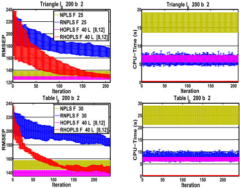
100 times, the acceleration rates are even higher with the larger numbers of latent vectors. Figure 2 shows that, for both scenarios, the predictive error of RHOPLS keeps decreasing at a faster rate as the iteration goes on, while the CPU cost remains as a low constant trend over time. We can also ob-
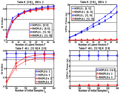
serve that, as illustrated in Figure 3, the prediction accuracy of RHOPLS stays very close to that of HOPLS as the number of latent vectors ranges from 10 to 90 for different loadings. However, the CPU time just slightly increases from 0.19s to 0.38s for RHOPLS with input loading [8, 12], which is in contrast to that of HOPLS from 1.79s to 19.22s, indicating the superior scalability of the RHOPLS with increasing number of latent vectors (d-ranks). The Q is given in Figure 3 with varying numbers of initial samples and mini-batch sizes. We may notice that only 50 initial samples, which is 8% of the whole training data, will suffice to guarantee a reasonably good result, i.e., nearly 0.78 for mini-batch size of 2.
| ECoG | Frequency 1hz X ∈ R900×10×10×16 | Frequency 5hz X ∈ R4500×10×10×16 | ||||||
|---|---|---|---|---|---|---|---|---|
| Methods | Hyper-parameters | Q | RMSEP | Time (s) | Hyper-parameters | Q | RMSEP | Time (s) |
| NPLS | F = 10 | .7014 (.0072) | 33.5 (0.7) | 3.15 (0.46) | F = 25 | .7338 (.0023) | 29.9 (0.4) | 28.6 (1.0) |
| RNPLS | F = 5, γ = 1 | .7096 (.0071) | 32.6 (0.6) | 1.70 (0.35) | F = 8, γ = 1 | .7197 (.0049) | 31.6 (0.5) | 4.87 (0.69) |
| HOPLS | F = 12 | .7336 (.0039) | 29.9 (0.4) | 1.86 (0.34) | F = 15 | .7343 (.0011) | 29.7 (0.2) | 9.07 (0.74) |
| IHOPLS | F = 10 | .7044 (.0082) | 33.1 (0.9) | 1.64 (0.32) | F = 10 | .7058 (.0086) | 33.0 (0.8) | 1.74 (0.48) |
| RHOPLS | F = 10 | .7308 (.0027) | 30.3 (0.3) | 0.16 (0.01) | F = 12 | .7330 (.0012) | 30.0 (0.2) | 0.20 (0.02) |
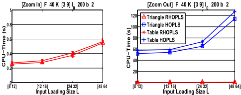
To see how all the methods behave in large "dimensionality" context, we fix the same hyper-parameters as in Table 1 but use frame size 240 × 320 instead of 24 × 32. Again, in Table 2, RHOPLS is quite close to HOPLS in accuracy but enormously enlarges the speed gaps against RNPLS and NPLS by more than 200 and 3000 times in "table" scenario, respectively. Figure 4 demonstrates the scalability of RHOPLS with increasing input loading size L. The right plot zooming in on the bottom of left plot shows that RHOPLS is much less sensitive to the growing loading size compared to HOPLS. This reflects the fact that the impact of large d-ranks on computational load when using HOPLS has been significantly diminished by using our feature-based updating strategy.
3.2 Neurotycho Electrocorticography Dataset
In this section, the tests were carried out on a benchmark tensor regression application, that is, decoding limb movements from monkey's brain signals using Neurotycho food tracking Electrocorticography (ECoG) dataset [Chao et al., 2010]. ECoG data contains a 15 minute-long recording and we downsampled motion data to different frequencies, producing various lengths of observations with different levels of overlapped features. As for the input, the wavelet transformed ECoG signal was represented as a 4th-order tensor (i.e., samples × time × frequency × channel). A 3rd-order tensor of 3D movement distances of the monkey's limb on 4 markers was used as the output. In Table 3, RHOPLS again performs consistently better than NPLS, RNPLS, IHOPLS for the 4th-order's input situation. In Figure 5, RHOPLS
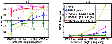
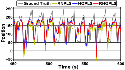
maintains nearly the same predictability with HOPLS in the settings of both low frequency (difficult case) and high frequency (easy case). In the meantime, RHOPLS consumes low CPU time regardless of the length of sequence, and exhibits high speed-up rates over RNPLS, i.e., 24 times faster at 4500, and overall nearly 10 times faster than IHOPLS, while NPLS and HOPLS are almost useless in fast time-critical applications. Note that the recursiveness property of RHOPLS implies that any long (even infinite) low-rank sequence can be handled by RHOPLS with a short constant processing time, thus we will get similar result for sequence with even larger "sample" complexity. Figure 6 visualizes an example of the observed and the predicted trajectories of monkey's hand.
4 Discussion
The drastic accelerations of our RHOPLS are realized in two stages, the first, due to Step 1, focuses on the reduction of "dimensionality" complexity. On the basis of the first stage, the second stage (i.e., Steps 2,3 and 4) concentrates on making the low constant "sample" complexity possible. The overall speed-ups stem from directly updating the set of factors (regression coefficients) in lightweight manner at a smallscale factor (feature) level instead of the raw data level, such that the relatively expensive eigenvector-style calculations are able to execute a lot faster on the factor scale.
@inproceedings{ijcai2017p257,
  title     = {Fast Recursive Low-rank Tensor Learning for Regression},
  author    = {Hou, Ming and Chaib-draa, Brahim},
  booktitle = {Proceedings of the Twenty-Sixth International Joint Conference on
               Artificial Intelligence, {IJCAI-17}},
  publisher = {International Joint Conferences on Artificial Intelligence Organization},
  editor    = {Carles Sierra},
  pages     = {1851--1857},
  year      = {2017},
  month     = {8},
  note      = {Main track},
  doi       = {10.24963/ijcai.2017/257},
  url       = {https://doi.org/10.24963/ijcai.2017/257},
}
TY - CPAPER TI - Fast Recursive Low-rank Tensor Learning for Regression AU - Hou, Ming AU - Chaib-draa, Brahim T2 - Proceedings of the Twenty-Sixth International Joint Conference on Artificial Intelligence, IJCAI-17 PB - International Joint Conferences on Artificial Intelligence Organization PY - 2017 SP - 1851 EP - 1857 DO - 10.24963/ijcai.2017/257 UR - https://doi.org/10.24963/ijcai.2017/257 ER -Copied
Machine-readable versions of this paper, for tools and AI agents:





