
Self-paced Mixture of Regressions
Proceedings of the Twenty-Sixth International Joint Conference on Artificial Intelligence. Main track. Pages 1816-1822.
https://doi.org/10.24963/ijcai.2017/252
Keywords
- Machine Learning: Data Mining
- Machine Learning: Machine Learning
Abstract
Mixture of regressions (MoR) is the well-established and effective approach to model discontinuous and heterogeneous data in regression problems. Existing MoR approaches assume smooth joint distribution for its good anlaytic properties. However, such assumption makes existing MoR very sensitive to intra-component outliers (the noisy training data residing in certain components) and the inter-component imbalance (the different amounts of training data in different components). In this paper, we make the earliest effort on Self-paced Learning (SPL) in MoR, i.e., Self-paced mixture of regressions (SPMoR) model. We propose a novel self-paced regularizer based on the Exclusive LASSO, which improves inter-component balance of training data. As a robust learning regime, SPL pursues confidence sample reasoning. To demonstrate the effectiveness of SPMoR, we conducted experiments on both the sythetic examples and real-world applications to age estimation and glucose estimation. The results show that SPMoR outperforms the state-of-the-arts methods.
- [Basso et al., 2010] Rodrigo M Basso, Víctor H Lachos, Celso Rômulo Barbosa Cabral, and Pulak Ghosh. Robust mixture modeling based on scale mixtures of skew-normal distributions. CSDA, 54(12):2926-2941, 2010.
- [Bennett et al., 2007] CM Bennett, M Guo, and SC Dhar- mage. Hba1c as a screening tool for detection of type 2 di- abetes: a systematic review. Diabetic Medicine, 24(4):333- 343, 2007.
- [Campbell and Allen, 2015] Frederick Campbell and Genev- era I Allen. Within group variable selection through the exclusive lasso. arXiv preprint arXiv:1505.07517, 2015.
- [Chamroukhi, 2016] Faicel Chamroukhi. Robust mixture of experts modeling using the t distribution. Neural Networks, 79:20-36, 2016.
- [Chang et al., 2011] Kuang-Yu Chang, Chu-Song Chen, and Yi-Ping Hung. Ordinal hyperplanes ranker with cost sensi- tivities for age estimation. In CVPR, 2011.
- [Cheng et al., 2016] Gong Cheng, Peicheng Zhou, and Jun- wei Han. Rifd-cnn: Rotation-invariant and fisher discrimi- native convolutional neural networks for object detection. In CVPR, 2016.
- [Geng et al., 2013] Xin Geng, Chao Yin, and Zhi-Hua Zhou. Facial age estimation by learning from label distributions. TPAMI, 35(10):2401-2412, 2013.
- [Guo and Mu, 2011] Guodong Guo and Guowang Mu. Simul- taneous dimensionality reduction and human age estimation via kernel partial least squares regression. In CVPR, 2011.
- [Guo and Mu, 2013] Guodong Guo and Guowang Mu. Joint estimation of age, gender and ethnicity: Cca vs. pls. In AFGR, 2013.
- [Guo et al., 2009] Guodong Guo, Guowang Mu, Yun Fu, and Thomas S Huang. Human age estimation using bio-inspired features. In CVPR, 2009.
- [Han et al., 2015] Hu Han, Charles Otto, Xiaoming Liu, and Anil K Jain. Demographic estimation from face images: Human vs. machine performance. TPAMI, 37(6):1148- 1161, 2015.
- [Hara and Chellappa, 2014] Kota Hara and Rama Chellappa. Growing regression forests by classification: Applications to object pose estimation. In ECCV, 2014.
- [Huang and Yao, 2012] Mian Huang and Weixin Yao. Mix- ture of regression models with varying mixing proportions: a semiparametric approach. JASA, 107(498):711-724, 2012.
- [Jacobs et al., 1991] Robert A Jacobs, Michael I Jordan, Steven J Nowlan, and Geoffrey E Hinton. Adaptive mix- tures of local experts. Neural computation, 3(1):79-87, 1991.
- [Jiang et al., 2014a] Lu Jiang, Deyu Meng, Teruko Mitamura, and Alexander G Hauptmann. Easy samples first: Self- paced reranking for zero-example multimedia search. In ACM MM, 2014. Jiang et al., 2014b] Lu Jiang, Deyu Meng, Shoou-I Yu, Zhenzhong Lan, Shiguang Shan, and Alexander Haupt- mann. Self-paced learning with diversity. In NIPS, 2014.
- [Jordan and Jacobs, 1994] Michael I Jordan and Robert A Ja- cobs. Hierarchical mixtures of experts and the em algorithm. Neural computation, 6(2):181-214, 1994.
- [Jordan and Xu, 1995] Michael I Jordan and Lei Xu. Conver- gence results for the em approach to mixtures of experts architectures. Neural networks, 8(9):1409-1431, 1995.
- [Kong et al., 2014] Deguang Kong, Ryohei Fujimaki, Ji Liu, Feiping Nie, and Chris Ding. Exclusive feature learning on arbitrary structures via ℓ 1,2 -norm. In NIPS, 2014.
- [Kumar et al., 2010] M Pawan Kumar, Benjamin Packer, and Daphne Koller. Self-paced learning for latent variable mod- els. In NIPS, 2010.
- [Lin, 2010] Tsung-I Lin. Robust mixture modeling using multivariate skew t distributions. SC, 20(3):343-356, 2010.
- [Nguyen and McLachlan, 2016] Hien D Nguyen and Geof- frey J McLachlan. Laplace mixture of linear experts. CSDA, 93:177-191, 2016.
- [Ricanek and Tesafaye, 2006] Karl Ricanek and Tamirat Tesafaye. Morph: A longitudinal image database of normal adult age-progression. In AFGR, 2006.
- [Song et al., 2014] Weixing Song, Weixin Yao, and Yanru Xing. Robust mixture regression model fitting by laplace distribution. CSDA, 71:128-137, 2014.
- [Supancic and Ramanan, 2013] James S Supancic and Deva Ramanan. Self-paced learning for long-term tracking. In CVPR, 2013.
- [Vijayakumar et al., 2017] Pavithra Vijayakumar, Robert G Nelson, Robert L Hanson, William C Knowler, and Mad- humita Sinha. Hba1c and the prediction of type 2 diabetes in children and adults. Diabetes Care, 40(1):16-21, 2017.
- [Young and Hunter, 2010] Derek S Young and David R Hunter. Mixtures of regressions with predictor-dependent mixing proportions. CSDA, 54(10):2253-2266, 2010.
- [Yuan and Lin, 2006] Ming Yuan and Yi Lin. Model selec- tion and estimation in regression with grouped variables. Journal of the Royal Statistical Society: Series B, 68(1):49- 67, 2006.
- [Zhang et al., 2016] Dingwen Zhang, Junwei Han, Chao Li, Jingdong Wang, and Xuelong Li. Detection of co-salient objects by looking deep and wide. IJCV, 120(2):215-232, 2016.
- [Zhang et al., 2017] Dingwen Zhang, Deyu Meng, and Jun- wei Han. Co-saliency detection via a self-paced multiple- instance learning framework. TPAMI, 39(5):865-878, 2017.
- [Zipf et al., 2013] George Zipf, Michele Chiappa, Kathryn S Porter, Yechiam Ostchega, Brenda G Lewis, and Jennifer Dostal. National health and nutrition examination survey: plan and operations, 1999-2010. Vital Health Stat 1, (56):1- 37, 2013.
References were extracted automatically from the PDF and may contain errors.
Full text extracted automatically from the PDF; figures, tables and equations may differ. The PDF is the version of record.
1 Introduction
Nonlinear regression is a longstanding problem in artificial intelligence community with enormous applications. The fundamental approaches extract feature representations from the data and learn a nonlinear function that maps the input features to the outputs, which fall into two main categories: (1) the universal approaches and (2) the divide and-conquer approaches.
Regression methods proposed in early ages are mainly the universal approaches. These methods fit data with universal nonlinear functions to whole data space such as the kernel function in Kernel Support Vector Regression [Guo et al., 2009] and Rectifier functions used in neural networks. These approaches can effectively improve the regression performance when facing the non-smooth data collection. However, when dealing with the piecewise continuous and heterogeneous data, they will be inevitably biased by data distribution: low regression error in densely sampled space while high error in everywhere else.
∗These authors contributed equally to this work.
†The corresponding author.
For addressing the issues of the data discontinuity and heterogeneity, the divide-and-conquer approaches were proposed lately. The core idea is to learn to combine multiple local regressors. For instance, the hierarchical-based [Han et al., 2015] and tree-based regression [Hara and Chellappa, 2014] make hard partitions recursively, and the subsets of samples may not be homogeneous for learning local regressors. While Mixture of Regressions (MoR) [Jacobs et al., 1991; Jordan and Xu, 1995] distributes regression error among local regressors by maximizing likelihood in the joint input-output space. These approaches reduce overall error by fitting regression locally and reliefs the bias by discontinuous data distribution.
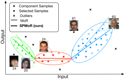
Unfortunately, the aforementioned approaches still cannot achieve satisfactory performance when applying in some realworld applications. The main reason is that these approaches tend to be sensitive to the intra-component outliers (i.e., the noisy training data residing in certain components) and the inter-component imbalance (i.e., the different amounts of training data in different components), which, however, happens to be two inherent properties of the exotic nature of the realworld data, i.e., nonuniform sampled and noisy (see Figure 1). For example, in the existing MoR approaches [Huang and Yao, 2012; Young and Hunter, 2010], regressors learnt from the components with more training data tend to dominant the other regressors in estimating the final output. In addition, regressors learnt with noisy training data tend to generate noisy mapping. These will inevitably prevent the learnt regression model from reaching to the global optimum.
| Standard LASSO | Group LASSO | Exclusive LASSO | |
|---|---|---|---|
| Norm Property Implication in SPL Reference | ℓ1 Global sparsity Selecting competing (confident) samples [Kumar et al., 2010] | ℓ2,1 or ℓ0.5,1 Inter-group sparsity Selecting samples from diverse groups [Jiang et al., 2014b; Zhang et al., 2017] | ℓ1,2 Intra-group sparsity and inter-group non-sparsity Selecting competing (confident) samples from diverse groups OURS |
To solve these two folds of problems, we make the earliest effort to introduce the self-paced learning (SPL) mechanism into the investigated regression problem and develop a novel Self-paced Mixture of regressions (SPMoR) model. The intuition behind SPL [Kumar et al., 2010] can be explained in its analogous to human education. A pupil is supposed to understand elementary algebra before he or she can learn more advanced algebra topics. In the past few years, the effectiveness of such learning regime has been validated in a number of tasks, like event detection [Jiang et al., 2014a] and co-saliency detection [Zhang et al., 2017]. SPL is essentially a robust learning regime: starting with easier aspects of a certain task and then gradually taking more complex examples into consideration, while the noisy examples are prevented from being used throughout the learning procedure. Consequently, it can be naturally used to screen the outliers during the learning procedure and thus address noisy data in regression. Notice that [Nguyen and McLachlan, 2016; Song et al., 2014; Basso et al., 2010; Lin, 2010] have also made efforts to build robust mixture models by using Laplace or t distribution, which do not consider conditional mixing proportions nor expand to the hierarchical framework. Compared with them, our SPMoR model overcome the sensitivity to the noisy data by introducing the effective self-paced regularizer rather than using certain types of data distribution.
Moreover, SPL is very flexible in designing task-specific regularizer. The most basic self-paced regularizer is the Standard LASSO [Kumar et al., 2010], i.e., the ℓ1 norm, which favors selecting sparse but competing training samples, i.e., samples with small training loss or high confidence. More recently, [Jiang et al., 2014b] and [Zhang et al., 2017] have additionally introduced the negative ℓ2,1 and negative ℓ0.5,1 norm into the self-paced regularizer. As two kinds of the Group LASSO [Yuan and Lin, 2006], ℓ2,1 and ℓ0.5,1 norm enforce the sparsity on variables at an intergroup level, where variables from different groups are competing to survive. Thus, their counter-part would discourage the inter-group sparsity and thus encourage the leaner to select diverse training samples residing in more groups. In this paper, we propose a novel self-paced regularizer, which is based on the Exclusive LASSO [Kong et al., 2014; Campbell and Allen, 2015]. Specifically, the Exclusive LASSO is formed by the ℓ1,2 norm, which encourages intragroup competition but discourages inter-group competition. The intra-group competition (sparsity) is achieved via ℓ1 norm, while inter-group non-sparsity, i.e., diversity, is achieved via ℓ2 norm. Consequently, it can be naturally used to build the robust mixture of regressions mechanism: On one hand, the encouraged intra-group competition will prevent the learner from using the outlier data within each component. On the other hand, the discouraged inter-group competition will induce the learner to select balanced training data from different components. A brief summarization of the properties of the Standard LASSO, Group LASSO, and Exclusive LASSO is shown in Table. 1. In sum, this paper present three major contributions:
- The earliest effort to use SPL to MoR, which effectively address the intra-component outlier and the intercomponent imbalance problem of the existing MoRs.
- A novel Exclusive LASSO based self-paced regularizer, which simultaneously encourages the intra-group competition and discourages inter-group competition.
- Significantly superior performance than other regression models and self-paced regulaizers on two real-word applications. To our knowledge, SPMoR achieves the best performance ever reported in literature on MORPH and NHANES datasets.
2 Mixture of Regressions
The standard MoR consists of a fully conditional mixture model where both the gating functions and the experts, are conditional on input features. Specifically, given xi ∈ ℜdx (the training sample) and yi ∈ ℜdy (the output vector), MoR splits the n pairs of samples {xi, yi}s into k components and learn a weighted linear regressor for each component.
The total probability of generating yi from input xi is the mixture of the the probabilities of generating yi from each component density, where the gating function provides multinomial probabilities. The conditional density of MoR is computed by summing over all local regressors:
where β = {β1, β2, · · · , βk}, w = {w1,w2, · · · ,wk}, σ = {σ1,σ2, · · · ,σk}, wj is the gating function parameter, βj ∈ ℜdy×(dx+1) is the regression coefficients, ˆx = [1, x], g(·) is the gating function, e.g., softmax function, which is positive and sum to 1, φ(·) is a density function of regression error, e.g., Gaussian error N(0, σ2 ). The output yi is estimated as a weighted combination over all local regressors:
The MoR model parameters are estimated by maximizing the observed data log-likelihood via using the EM algorithm. The observed data log-likelihood for the parameter vector is
For optimizing (3), the E-Step at each iteration of the EM algorithm requires the calculation of the following posterior probability zij that the sample (xi, yi) belongs to the j th expert, given a parameter estimation wj, βj and σj. Then, the M-step calculates the parameter update wj, βj and σj by maximizing the expected complete-data log-likelihood for each expert where zij is fixed.
3 SPMoR
Without loss of generality, we introduce the method to obtain SPMoR by integrating the proposed self-paced regularizer with the standard MoR model. By using the proposed method, we can also integrate the self-paced regularizer with the stronger hierarchical mixture of experts model [Jordan and Jacobs, 1994], which obtains the SPMoR+ model by using Bayes' rule 1 .
3.1 The Object Function
We establish a novel SPMoR framework by introducing the Exclusive LASSO-based self-paced regularizer into the learning objective:
where vij ∈ {0, 1} is the learning weight of each training sample, which represents whether the sample xi has been selected by self-paced learning for j th component. ||V||21 = ∑kj=1 (||vj||1)2 is the Exclusive LASSO, which is a combination of the ℓ1 and ℓ2 norms. Specifically, the Exclusive LASSO is originally used for variable selection, where the structured variable selection problem can be phrased as a constrained optimization problem where loss function is minimized subject to a constraint that ensures sparsity and selects at least one variable from every group. Inspired by this, we introduce the Exclusive LASSO to perform structured sample selection in learning MoR. It seeks to accurately learn the mixture model by using a set of "easy" samples from each component rather than using all the training data. "Easy" samples in this case
1 The joint posterior probability is the product of the conditional posterior probabilities along path from the root to the experts in ( 1).
Algorithm 1 SPMoR Training Algorithm
Require: Given training samples xi, yi (i = 1, · · · , n):
- Initialize the number of the regression k.
- Do k-means clustering on {xi, yi}s to get k subsets, and initialize zij according to cluster label, i.e. zij = 1 if xi is assigned to the j th cluster, otherwise zij = 0.
- Use samples in each subset to initialize the gate function parameters wj , and local regressor parameters βj , and σ2 j . 4. implement the generalized EM algorithm:
for each iteration do
- Calculate the zij in E-Step (Eq. 5);
- Update thevij, wj, βj, and σ2 j in M-Step;
for each component do
- (1. Fix parameter zij, wj, βj, and σ2 j , compute the log-likelihood value lij for xi by Eq. 8, and sort lij in descent order;
- (2. For all r = 1, . . . , n, if lrj ≥ λ(2r - 1), then set vrj = 1, otherwise, vrj = 0.
- (3. Fix parameter zij and vij, update parameters wj, βj, and σ2 j by Eq. 12, 13 and 14.
end for
end for
- Repeat until convergence.
refers to the samples having high likelihood value. Basically, when λ is small, only the samples with high likelihood, gate probability is close to 1, and density is larger than 1, will be chosen as training data. Thus, the learning objective (4) can on one hand help improving the balance of the selected training data among different components, and on the other hand, screening most of the outliers in each component.
Notice that (4) has some distinct properties as compared with the existing SPL formulations [Jiang et al., 2014b; Zhang et al., 2017]. Specifically, in our formulation, by setting λ to 0, i.e., only introducing the sample weight parameter V without any self-paced regulzier, the SPMoR would already enable the learner to select "easy" training samples, i.e., the samples with φ(yi|βT j ˆ xi, σ2 j ) > 1. However, in [Jiang et al., 2014b; Zhang et al., 2017], the learner won't have such capacity and it won't select any training sample in this case. In addition, instead of obtaining the data group solely based on clustering [Jiang et al., 2014b] or using physical constraint [Zhang et al., 2017], we propose a unified framework to jointly infer the expert components as the data groups and learn the local regressors in each components.
3.2 The Optimization
To maximize log-likelihood function (4), the generalized EM algorithm starts from an initial parameter vector and alternates between E-step and M-step until convergence. The E-step computes the expected completed data log-likelihood and the M-step maximizes it. The pseudo code of the SPMoR training algorithm is summarized in Algorithm 1.
E-Step
Similar with the standard MoR, we compute the posterior probability zij of function 4 in the E-step. Specifically, given the initial parameters, we can obtain
where vij indicates that whether the sample is chosen by selfpaced learning. If vij = 0 for all the components, then the sample is eliminated from training procedure. If all vij = 1, it is the same as the function of the conventional MoR.
M-step
In M-step, we fix zij and utilize the alternative convex search (ACS) to alternatively optimizes w, β, σ and V.
Updating Self-paced Parameter:
Firstly, we fix the parameters w, β, σ of the gating function and local regressors to optimize V as following
where V ∈ ℜn×k , each element vij in the matrix indicates the sample xi's "easiness" in j th component. Here, "easiness" means the confidence of the sample, which indicates whether the sample should be used for training. By contrast, zij indicates the probability that sample belongs to j th component.
It is easy to see that the original problem (6) can be equivalently decomposed as a series of the following suboptimization problems (j = 1, . . . , k):
which means that vj(r) is the optimum of function (7) if it is further constrained to be with r nonzero entries. It is then easy to deduce thatv⋆
Then let's calculate the difference between any two adjacent elements in the sequence E(vj(r)).
Here, we sort the log-likelihood values in the j th component in descent order. Then, lij is a monotonically decreasing sequence with r, while 2r + 1 is a monotonically increasing sequence. So diffr is a monotonically decreasing sequence. When diffr → 0 and diffr > 0, we can get the function E(vj(r)) is increasing more and more slowly. When diffr < 0, the log-likelihood value will be decreasing. Therefore, in function (11) E(vj(r)) will get the maximum value when diffr = 0. Finally, we can get the optimal solution for vj in j th component. For all r = 1, . . . , n, if lrj > λ(2r - 1), then vrj = 1; otherwise, vrj = 0.
Updating MoE parameter: After updating the self-paced parameter V, we can fix vij and zij to update the MoE parameters w, β and σ. Here, we use Iteratively Reweighted Least Squares (IRLS) algorithm [Jordan and Jacobs, 1994] to update the gating function and experts function:
1) For the j th gating function, the gradient of any sample xi is obtained by:
2) For the j th regression coefficients, the gradient is obtained by:
and the corresponding variance σj is obtained by:
Given a test input xt ∈ ℜdx , the output of SMMR, yt ∈ ℜdy , is computed as (15).
4 Experiments
4.1 Simulation
We conducted simulation experiments in two settings to demonstrate the effectiveness of the proposed algorithm.
Setting 1: In this experiment we mainly examine the robustness of the proposed model to outliers by comparing with the standard MoR and another two existing robust MoR methods. Specifically, we followed the same settings with [Chamroukhi, 2016] to generate the simulated data: we simulated 500 observations from a k = 2 component MoR with (1), where the parameter components were w1 = (0, 10)T , w2 = (0, 0)T , β1 = (0, 1)T , β2 = (0,-1)T and σ1 = σ2 = 0.1. The feature xi was simulated uniformly over interval (-1, 1). Outliers (0% - 5% of 500 observations) were also generated by simulating xi uniformly over the interval (-1,1), while setting y = -2. To assess robustness, the mean squared error (MSE) between each component of the true parameter vector and the estimated one, were averaged on 100 trails and reported in Table 2. As it can be observed, the parameter estimation error of our method (SPMoR) can stay in relative smaller values, which demonstrates the robustness of the proposed algorithm outperforms the existing robust MoR methods.
| Method | 0% | 1% | 2% | 3% | 4% | 5% | Avg. |
|---|---|---|---|---|---|---|---|
| MoE [Jacobs et al., 1991] | 0.000178 | 0.001057 | 0.001241 | 0.003631 | 0.013257 | 0.028966 | 0.008055 |
| LMoE [Nguyen and McLachlan, 2016] | 0.000144 | 0.000389 | 0.000686 | 0.000153 | 0.000296 | 0.000121 | 0.000298 |
| TMoE [Chamroukhi, 2016] | 0.000168 | 0.000566 | 0.000464 | 0.000221 | 0.000263 | 0.000045 | 0.000288 |
| SPMoR(ours) | 0.000091 | 0.000269 | 0.000277 | 0.000202 | 0.000112 | 0.000101 | 0.000175 |
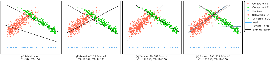
Setting 2: In this experiment, we subjectively evaluated the effectiveness of the proposed algorithm. The data used for this simulation were generated basically following the same way as in the Setting 1, expect for two components were generated with different amount of observations and variances. The experimental results are shown in Figure 2, from which we can observe that due to the intra-component outliers and the inter-component imbalance, the initial regressors as well as the standard MoR cannot fit to the data well. Whereas along the learning iteration, our algorithm (SPMoR) can gradually revise the local regressors by inferring the reliable training data from each component (i.e., the red/green dots in Figure 2). Finally, the regression result of our algorithm converges to the solution that is close to the ground-truth.
As can be seen from Figure 2, with a feasible λ, it seeks to select more even set of "easy" samples from each component. Specifically, in each iteration, it prefers to select the confidant samples which are the easy-separable points with small regression-errors. So the posterior probabilities zij for the selected samples tend to be equal to 1, which makes the variance σj for each component is similar and small. Consequently, the learner tends to select samples within similar and small bandwidth from each component (shown as the red/green dots in the Figure 2), which leads to the increase of the balance of the selected training data.
4.2 Age Estimation
Given a collection of human face images, the goal is to determine the specific ages of the subjects shown in the corresponding face images, solely based on the image content. The task is very challenging due to the complex pattern structure, which not only caused by intrinsic factors, e.g. genetic factors, but also by extrinsic factors, e.g. expression, and environment.
Dataset: We conducted experiments on the most frequently used Longitudinal Morphological Face Database (MORPH) [Ricanek and Tesafaye, 2006] database, which contains 55,132 face images frommore than 13, 000 subjects. The ages of the subjects range from 16 to 77 with a median age of 33. The faces are from different races, including African, European, Hispanic, Asian, Indian, et al.
Experimental settings: We used the 4,376 BIF features [Guo et al., 2009] 2 to represent each image and followed [Geng et al., 2013] to reduce the feature dimension to 200 by using the marginal Fisher analysis. Note that both SPMoR and SPMoR+ used softmax in partition and linear local regressors. In SPMoR, we set k to 9, and λ to 1e-05. In SPMoR+, we set k to 8, and λ to 1e-05. The SPMoR+ approach will be converged after 70 iterations, The running time of our method is 565 seconds, which is faster than HME which needs 48 iterations but costs 589 seconds.
2 thank Dr. Guodong Guo for providing the BIF features of the MORPH database.
| Method | Mean Absolute Error |
|---|---|
| CPNN [Geng et al., 2013] | 4.87 |
| CCA [Guo and Mu, 2013] | 4.73 |
| KPLS [Guo and Mu, 2011] | 4.43 |
| LSVR [Guo et al., 2009] | 4.31 |
| OHRank [Chang et al., 2011] | 3.82 |
| HSVR [Han et al., 2015] | 3.60 |
| SPMoR+(ours) | 3.55 |
In our experiment, we compared with the six state-of-thearts and four baseline models (see Table. 3 and Table. 4 for concrete references). All the comparisons were based on the same BIF feature and followed the same experimental protocols: randomly dividing the whole dataset into two parts: 80% for training and the other 20% for test, and repeating 30 random trails. Next, in the first run, the optimal hyper-parameters, including k and λ, were obtained by using grid-search with tenfold CV on the training set. To ensure the fair performance of the trained model, another 29 runs were conducted with the same parameters. All results were evaluated by Mean Absolute Error (MAE).
Results: The comparison results with the state-of-the-art age estimation on the MORPH dataset were reported in Table 3, from which we can observe that the proposed SPMoR+, i.e.,the "ours" shown in the table, can obtain more promising performance. Specifically, compared with the universal nonlinear regression methods, such as KPLS [Guo and Mu, 2011] and LSVR [Guo et al., 2009], our regression model was learnt in a divide-and-conquer fashion, which can better address the issues of the data heterogeneity. While, compared with the existing divide-and-conquer nonlinear regression methods, such as HSVR [Han et al., 2015], our regression model was learnt under the guidance of a novel self-paced learning regime, which can further address the issues of the intra-component outliers and the inter-component imbalance of the data. For evaluating the sensitivity of the parameters on SPMoR+, we firstly fix k to 4, and set lambda to 1e-05,1e-04 and 1e-03. The corresponding MAEs obtained on MORPH dataset are 3.67, 3.88, 3.94. Then we set k to 4 and 8, and fix lambda to 1e-05. The obtained MAEs are 3.67 and 3.55.
To further demonstrate the effectiveness of the proposed self-paced regularizer, we reported the comparison results with four baseline models as in Table. 4. The comparison between MoE and SPMoR as well as the comparison between HME
| Method | Mean Absolute Error |
|---|---|
| MoE [Jacobs et al., 1991] | 3.83 |
| HME [Jordan and Xu, 1995] | 3.69 |
| HME+ℓ1 [Kumar et al., 2010] | 3.65 |
| HME+ℓ2,1 [Jiang et al., 2014b] | 3.62 |
| SPMoR(ours) | 3.76 |
| SPMoR+(ours) | 3.55 |
and SPMoR+ demonstrate that introducing the proposed selfpaced regularizer can significantly improve the performance of the corresponding base regression model. While, the comparison among HME+ℓ1 [Kumar et al., 2010], HME+ℓ2,1 [Jiang et al., 2014b], and SPMoR+ demonstrate the superior capability of the proposed Exclusive LASSO-based self-paced regularizer as compared with the existing ones.
4.3 Glucose Estimation
Given a collection of cohort data, the goal is to estimate the Glycated Hemoglobin HbA1c [Bennett et al., 2007], which can reflect the level of glucose [Vijayakumar et al., 2017] for undiagnosed type 2 Diabetes patients.
Dataset: We conducted experiments on the popular 20092014 National Health and Nutrition Examination Survey (NHANES) dataset [Zipf et al., 2013], which is the crosssectional data and the ground-truth HbA1c data were publicly available. The amount of all available data is 8,271. In specific, 15 features of NHANES data have been included into the model under routine health examination through a questionnaire on health behavior and clinical measurements.
Experimental settings: In this experiment, we compared our approach with 6 baseline models under the same protocol of Age Estimation. We randomly shuffled the dataset 100 times, and divided the data into two parts: 80% for training and the other 20% for test. All the results were evaluated by Mean Squared Error (MSE) and the Standard Deviation (S.D.). In SPMoR, we set k to 5, and λ to 1e-05. In SPMoR+, we set k to 16, and λ to 1e-04.
Results: The experimental results on the NHANES dataset were shown in Table 5. From which we can observe that the proposed SPMoR+ obtains the most state-of-the-art performance. To be more specific, the universal nonlinear method SVR cannot obtain the performance as good as the other divide-and-conquer models, while the hierarchical methods generally obtain better performance than the single mixure model. In addition, consistent with the experimental results in Sec. 4.2, the comparison between MoE and SPMoR and the comparison between HME and SPMoR+ demonstrate the effectiveness of the proposed framework to introduce self-paced learning into the regression problem. Finally, the comparison between HME+ℓ1, HME+ℓ2,1, and SPMoR+ demonstrates the superior performance of the proposed Exclusive LASSObased self-paced regularizer.
| Method | MSE ± S.D. |
|---|---|
| Support Vector Regression | 0.510 ± 0.02 |
| Gaussian Mixture Regression | 0.338 ± 0.01 |
| MoE [Jacobs et al., 1991] | 0.349 ± 0.01 |
| HME [Jordan and Xu, 1995] | 0.312 ± 0.05 |
| HME+ℓ1 [Kumar et al., 2010] | 0.293 ± 0.06 |
| HME+ℓ2,1 [Jiang et al., 2014b] | 0.292 ± 0.05 |
| SPMoR(ours) | 0.346 ± 0.01 |
| SPMoR+(ours) | 0.279 ± 0.03 |
5 Conclusion
We have proposed a novel SPL-based framework to effectively overcome limitations of MoR under nonuniform sampled and noisy real-world data. To our knowledge, this is the earliest effort to build self-paced regularizer based on the Exclusive LASSO, and to directly avoid the intra-component outlier and the inter-component imbalance problems in existing MoR approaches. Comprehensive experiments on the simulation data and two real-world tasks have demonstrated the effectiveness of the proposed approach. In the future, we will explore soft weighting regularizers in MoRs and appliy our approach in more computer vision tasks like object tracking [Supancic and Ramanan, 2013], co-saliency detection [Zhang et al., 2016], and object detection [Cheng et al., 2016].
@inproceedings{ijcai2017p252,
  title     = {Self-paced Mixture of Regressions},
  author    = {Han, Longfei and Zhang, Dingwen and Huang, Dong and Chang, Xiaojun and Ren, Jun and Luo, Senlin and Han, Junwei},
  booktitle = {Proceedings of the Twenty-Sixth International Joint Conference on
               Artificial Intelligence, {IJCAI-17}},
  publisher = {International Joint Conferences on Artificial Intelligence Organization},
  editor    = {Carles Sierra},
  pages     = {1816--1822},
  year      = {2017},
  month     = {8},
  note      = {Main track},
  doi       = {10.24963/ijcai.2017/252},
  url       = {https://doi.org/10.24963/ijcai.2017/252},
}
TY - CPAPER TI - Self-paced Mixture of Regressions AU - Han, Longfei AU - Zhang, Dingwen AU - Huang, Dong AU - Chang, Xiaojun AU - Ren, Jun AU - Luo, Senlin AU - Han, Junwei T2 - Proceedings of the Twenty-Sixth International Joint Conference on Artificial Intelligence, IJCAI-17 PB - International Joint Conferences on Artificial Intelligence Organization PY - 2017 SP - 1816 EP - 1822 DO - 10.24963/ijcai.2017/252 UR - https://doi.org/10.24963/ijcai.2017/252 ER -Copied
Machine-readable versions of this paper, for tools and AI agents:





