
Understanding Users' Budgets for Recommendation with Hierarchical Poisson Factorization
Proceedings of the Twenty-Sixth International Joint Conference on Artificial Intelligence. Main track. Pages 1781-1787.
https://doi.org/10.24963/ijcai.2017/247
Keywords
- Machine Learning: Data Mining
- Uncertainty in AI: Approximate Probabilistic Inference
- Machine Learning: Learning Preferences or Rankings
- Machine Learning: Learning Graphical Models
Abstract
People consume and rate products in online shopping websites. The historical purchases of customers reflect their personal consumption habits and indicate their future shopping behaviors. Traditional preference-based recommender systems try to provide recommendations by analyzing users' feedback such as ratings and clicks. But unfortunately, most of the existing recommendation algorithms ignore the budget of the users. So they cannot avoid recommending users with products that will exceed their budgets. And they also cannot understand how the users will assign their budgets to different products. In this paper, we develop a generative model named collaborative budget-aware Poisson factorization (CBPF) to connect users' ratings and budgets. The CBPF model is intuitive and highly interpretable. We compare the proposed model with several state-of-the-art budget-unaware recommendation methods on several real-world datasets. The results show the advantage of uncovering users' budgets for recommendation.
- [Blei et al., 2016] David M Blei, Alp Kucukelbir, and Jon D McAuliffe. Variational inference: A review for statisti- cians. arXiv preprint arXiv:1601.00670, 2016.
- [Chaney et al., 2015] Allison JB Chaney, David M Blei, and Tina Eliassi-Rad. A probabilistic model for using social networks in personalized item recommendation. In Pro- ceedings of the 9th ACM Conference on Recommender Systems, pages 43-50. ACM, 2015.
- [Charlin et al., 2015] Laurent Charlin, Rajesh Ranganath, James McInerney, and David M Blei. Dynamic poisson factorization. In Proceedings of the 9th ACM Conference on Recommender Systems, pages 155-162. ACM, 2015.
- [Du and Kamakura, 2008] Rex Y Du and Wagner A Ka- makura. Where did all that money go? understanding how consumers allocate their consumption budget. Journal of Marketing, 72(6):109-131, 2008.
- [Goldberg et al., 1992] David Goldberg, David Nichols, Brian M Oki, and Douglas Terry. Using collaborative fil- tering to weave an information tapestry. Communications of the ACM, 35(12):61-70, 1992.
- [Gopalan et al., 2013] Prem Gopalan, Jake M Hofman, and David M Blei. Scalable recommendation with poisson fac- torization. arXiv preprint arXiv:1311.1704, 2013.
- [Gopalan et al., 2014] Prem K Gopalan, Laurent Charlin, and David Blei. Content-based recommendations with poisson factorization. In Advances in Neural Information Processing Systems, pages 3176-3184, 2014.
- [Gourinchas and Parker, 2002] Pierre-Olivier Gourinchas and Jonathan A Parker. Consumption over the life cycle. Econometrica, 70(1):47-89, 2002.
- [Hoffman et al., 2013] Matthew D Hoffman, David M Blei, Chong Wang, and John William Paisley. Stochastic varia- tional inference. Journal of Machine Learning Research, 14(1):1303-1347, 2013.
- [Jordan et al., 1999] Michael I Jordan, Zoubin Ghahramani, Tommi S Jaakkola, and Lawrence K Saul. An introduc- tion to variational methods for graphical models. Machine learning, 37(2):183-233, 1999.
- [Kao et al., 2001] Chihwa Kao, Lung-fei Lee, Mark M Pitt, et al. Simulated maximum likelihood estimation of the lin- ear expenditure system with binding non-negativity con- straints. Annals of Economics and Finance, 2(1):203-223, 2001.
- [Kooti et al., 2016] Farshad Kooti, Kristina Lerman, Luca Maria Aiello, Mihajlo Grbovic, Nemanja Djuric, and Vladan Radosavljevic. Portrait of an online shopper: Understanding and predicting consumer behavior. In Proceedings of the Ninth ACM International Conference on Web Search and Data Mining, pages 205-214. ACM, 2016.
- [Koren and Bell, 2011] Yehuda Koren and Robert Bell. Ad- vances in collaborative filtering. In Recommender systems handbook, pages 145-186. Springer, 2011.
- [Koren et al., 2009] Yehuda Koren, Robert Bell, Chris Volin- sky, et al. Matrix factorization techniques for recom- mender systems. Computer, 42(8):30-37, 2009.
- [Koren, 2008] Yehuda Koren. Factorization meets the neigh- borhood: a multifaceted collaborative filtering model. In Proceedings of the 14th ACM SIGKDD International Con- ference on Knowledge Discovery and Data Mining, pages 426-434. ACM, 2008.
- [Kyrola et al., 2012] Aapo Kyrola, Guy Blelloch, and Carlos Guestrin. Graphchi: large-scale graph computation on just a pc. In Presented as part of the 10th USENIX Symposium on Operating Systems Design and Implementation (OSDI 12), pages 31-46, 2012.
- [McAuley and Leskovec, 2013] Julian McAuley and Jure Leskovec. Hidden factors and hidden topics: understand- ing rating dimensions with review text. In Proceedings of the 7th ACM Conference on Recommender Systems, pages 165-172. ACM, 2013.
- [Rendle et al., 2009] Steffen Rendle, Christoph Freuden- thaler, Zeno Gantner, and Lars Schmidt-Thieme. Bpr: Bayesian personalized ranking from implicit feedback. In Proceedings of the twenty-fifth conference on uncertainty in artificial intelligence, pages 452-461. AUAI Press, 2009.
- [Resnick and Varian, 1997] Paul Resnick and Hal R Varian. Recommender systems. Communications of the ACM, 40(3):56-58, 1997.
- [Salakhutdinov and Mnih, 2008a] Ruslan Salakhutdinov and Andriy Mnih. Bayesian probabilistic matrix factoriza- tion using markov chain monte carlo. In Proceedings of the 25th International Conference on Machine Learning, pages 880-887. ACM, 2008.
- [Salakhutdinov and Mnih, 2008b] Ruslan Salakhutdinov and Andriy Mnih. Probabilistic matrix factorization. In Advances in Neural Information Processing Systems, volume 20, 2008.
- [Shi et al., 2012] Yue Shi, Alexandros Karatzoglou, Linas Baltrunas, Martha Larson, Nuria Oliver, and Alan Han- jalic. Climf: learning to maximize reciprocal rank with collaborative less-is-more filtering. In Proceedings of the sixth ACM conference on Recommender systems, pages 139-146. ACM, 2012.
- [Xie et al., 2010] Min Xie, Laks VS Lakshmanan, and Pe- ter T Wood. Breaking out of the box of recommenda- tions: from items to packages. In Proceedings of the fourth ACM conference on Recommender systems, pages 151- 158. ACM, 2010.
References were extracted automatically from the PDF and may contain errors.
Full text extracted automatically from the PDF; figures, tables and equations may differ. The PDF is the version of record.
1 Introduction
Online market is expanding to an unparalleled scale. Facilitated by websites such as Amazon.com and Alibaba.com, people more and more rely on online shopping and consume millions of products every day. This is accompanied with the rapid increase of the online retail. In 2010, the Internet economy accounts for 4.7% of the US gross domestic product (GDP) while in 2016 the contribution has increased to 5.4% 1 . And the proportion of the online retail tends to continue to rise in the years ahead. This phenomenon inevitably has a big impact on every aspects of our life.
With the growth of the online market, there is an urgent need for intelligent recommendation of products for customers. Most of the online shopping websites leverage recommender systems to record users' usage data such as ratings and clicks to uncover their latent preferences. However, most of the recommendation algorithms are budgetunaware, in other words, they cannot avoid recommending users with products that exceed their budgets and they also cannot understand how users will assign their budgets to different products. According to [Du and Kamakura, 2008], consumers allocate their budgets by considering both the "whether to spend" and the "how much to spend" decisions to maximize the utility function. Thus the consumers' decisions imply an unified preference structure for different products within a category. In this paper, we propose a model called collaborative budget-aware Poisson factorization (CBPF) to consider users' ratings and budgets simultaneously. With the understanding of how users' budgets affect their purchasing behaviors, we can provide more intelligent recommendations. Few works in recommender systems community consider the monetary limit of users. To the best of our knowledge, this is the first work that considers modeling users' budgets in a generative way for product recommendation.
∗Corresponding author.
1 https://www.bcg.com/documents/file100409.pdf
Why try to model users' budgets? Unlike the category of books or movies, price plays a more important role in affecting users' purchases of commercial goods such as cellphones or jewelries. As pointed out by [Du and Kamakura, 2008; Kooti et al., 2016], users usually have finite budgets and they will assign more budgets to the products that they prefer. So to understand how the users will divide their budgets across different products is of great practical importance. Moreover, some users may put more budgets on certain kinds of product attributes. For example, some customers may willing to pay extra budgets for a larger cellphone screen compared with a powerful battery. All these phenomena demonstrate the rationality and importance of uncovering users' budgets for intelligent item recommendation. This is a blind spot of traditional recommender systems.
Why model with Poisson factorization? Hierarchical Poisson factorization (HPF) [Gopalan et al., 2013] is an effective item recommendation model for users' ratings. It has been used for content-based recommendation [Gopalan et al., 2014], social-based recommendation [Chaney et al., 2015] and dynamic recommendation [Charlin et al., 2015]. There are three reasons for modeling users' budgets based on HPF. First is that HPF can be interpreted as a two-stage process that the user first decides a budget, then allocates this budget accross different products. This interpretation makes HPF intuitive to model the process of users' allocation of budgets. Second is that previous works [Gopalan et al., 2013; Chaney et al., 2015] point out HPF is better than Gaussian matrix factorization based models [Salakhutdinov and Mnih, 2008a; 2008b] in estimating users' activity levels. Third is that the inference of HPF is generally fast due to it only relies on the observed cells of the feedback matrix.
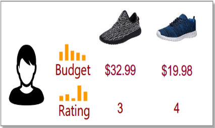
Case study: In Figure 1, we take a user's purchasing records as an example. The user bought two shoes from Amazon.com. He spent more on the first one but rated it lower. So from the perspective of preference-based recommender systems, the user preferred the second shoe to the first. On the other hand, from the perspective of budget-aware recommendation, since the user spent more on the first shoe, he preferred the first shoe to the second. That means the first shoe has some properties that the user preferred and decided to allocate more funds. This reflects that the products the users actually bought do not necessarily cost less. If the user spent a lot on a product, this means the user preferred the product to other products. So in generally users will buy products that they both prefer and afford. The ratings the user given to the products and the budget the user allocated to the products are both indicators of the user's inclinations. Thus for intelligent recommendation, it is crucial to take both perspectives into consideration.The orange bars represent the latent vector representations of users' preferences. The height of the bars means what attribute the user will assign more budget and how the user will rate the attribute accordingly.
Summary and contributions: In this paper, we develop a generative model named collaborative budget-aware Poisson factorization (CBPF) to connect users' ratings and budgets simultaneously. The model is intuitive and highly interpretable. The contributions of the paper are summarized below:
- We propose a generative model to connect users' ratings and budgets in a cohesive manner.
- We develop an efficient variational inference optimization algorithm to approximate the posterior distribution of the model.
- The experimental results reveal the advantage of the proposed model compared with state-of-the-art budgetunaware recommendation models.
2 RelatedWork
Recommender systems have drawn more attentions from the machine learning community since the emergence of the e-commerce [Resnick and Varian, 1997]. Various approaches have been proposed to provide better product recommendations. Among them, collaborative filtering [Goldberg et al., 1992; Koren, 2008; Koren and Bell, 2011] is a leading technique which tries to recommend a user with products by analysing similar users' records. Gaussian matrix factorization models [Salakhutdinov and Mnih, 2008a; 2008b] were proposed recently to handle extremely large datasets and to deal with cold-start users who have very few ratings. In matrix factorization models, users and items are represented as low-dimensional vectors. The latent user vectors indicate user preferences and latent item vectors indicate item attributes. This representation is also called latent factor model [Koren, 2008; Koren et al., 2009].
In order to better handle the data sparsity problem and the long-tail of users and items, hierarchical Poisson factorization [Gopalan et al., 2013] was proposed recently to be an alternative to Gaussian matrix factorization models. The main problem with Gaussian matrix factorization models is that they systematically overestimate users' activity levels [Gopalan et al., 2013]. Recently, many variants of hierarchical Poisson factorization model [Gopalan et al., 2014; Chaney et al., 2015; Charlin et al., 2015] were developed to provide more flexible item recommendations.
Understanding how budgets affect users' purchasing decisions is an important topic in the field of economics [Kao et al., 2001; Gourinchas and Parker, 2002; Du and Kamakura, 2008]. However, all these works are taken from an economical perspective. Based on our analysis above, uncovering users' budgets can also be an important issue in the field of recommender systems. However, few works consider incorporating budgets into recommender systems. [Xie et al., 2010] considers the situation that users choose a travel package on a limited budget. To the best of our knowledge, this paper is the first one that works on incorporating users' budgets into recommender systems in a generative way.
3 Preliminaries
3.1 ProblemDefinition and Notations
In this paper, we assume that there are U users and V items. Following the convention of latent factor models, we represent each entity as a low-dimensional latent vector and the latent dimension is denoted as K. For a user u, we represent the latent assignment vector as φu, which indicates how the user will assign the budget to different item attributes. And we denote the latent rating vector as θu, which indicates how the user will rate each item attribute. So the orange bars in Figure 1 are illustrations of φu and θu. Meanwhile, the latent attribute vector of item v is denoted as βv. The monetary allocation of the user u to item v is puv and the rating that the user u give to item v is yuv.
We denote the observed feedback (the set of products that the user bought) of user u as Ou. For each unseen item v (the product that the user did not buy) of the user u, the task of a recommendation model m is to construct a ranking score fu(v) based on Ou and then recommend the user with items with high ranking scores.
3.2 Hierarchical Poisson Factorization
Hierarchical Poisson factorization [Gopalan et al., 2013] is a probabilistic collaborative filtering recommendation model for users' ratings. In hierarchical Poisson factorization, users and items are represented as low-dimensional and nonnegative sparse vectors. The latent user vectors indicate user preferences and the latent item vectors indicate item attributes. The ratings that users give to items are assumed to be drawn from Poisson distributions. The rate of the Poisson distribution is set to be the inner product of the latent user vector and latent item vector. Meanwhile, each component of the latent user vector and the latent item vector is drawn from a Gamma distribution whose rate is assumed to be drawn from another Gamma distribution with fixed parameters.
4 ProposedModel
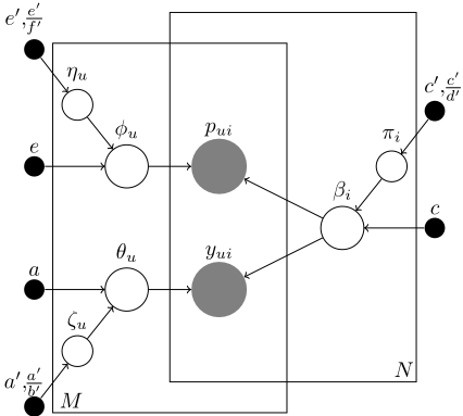
In CBPF, we try to uncover how users will assign their budgets to each item attribute and how users will rate the attribute accordingly. Unlike HPF [Gopalan et al., 2013] which only considers users' ratings, we model users' ratings and budgets in a cohesive manner which captures the intuition that for intelligent recommendation it is important to involve users' budgets. The generative process of HPF is similar to CBPF and we omit it due to space limitation. Based on above analysis, the generative process of CBPF is defined as follows:
- For each user u:
- (a) Sample ζu ∼Gamma(a′ ,a′ /b′ ).
- (b) For each component k, sample preference
- (c) Sample πu ∼Gamma(e′ ,e′ /f ′ ).
- (d) For each component k, sample assignment
- For each item v:
- (a) Sample ηu ∼Gamma(c′ ,c′ /d′ ).
- (b) For each component k, sample attribute
- For each user u and item v,
- (a) sample rating
- (b) sample allocation
In this paper, we use budget to refer to the monetary limit of a user, which equals to the sum of all allocations. The monetary allocation of the user u to item v is just the price of item v. And we use assignment to refer to the monetary allocation to a particular item attribute. So the latent assignment vector φu indicates how the user u will allocate her budget to different item attributes. The allocation puv of user u for item v is assumed to be drawn from a Poisson distribution whose rate is the inner product of the latent assignment vector and the latent attribute vector.
Users' ratings and allocations are highly correlated and both stem from the interaction of user preferences and product attributes. In CBPF, they are coupled in a natural and cohesive manner. HPF is a special case of the proposed model which only considers users' ratings. The latent variables of CBPF are θ1:U , φ1:U , β1:V , ζ1:U , π1:V and η1:U . The observed variables are users' ratings y and users' allocations p.
Interpretation: Due to the relation between Poisson distribution and multinomial distribution, we can re-write the generative process of users' allocations as a two-stage procedure similar to [Gopalan et al., 2013]. The user u first decides an amount of budget bu and then chooses how to allocate the budget across different products:
This interpretation makes it intuitive to model users' budgets with Poisson distribution. Moreover, the non-negative constraint of the latent assignment vectors makes it practically reasonable to model users' assignments of budgets.
Recommending new products: To recommend new products for each user, we fit the posterior distribution p(ζ1:U, θ1:U, π1:V , β1:V , η1:U, φ1:U|y, p) using a variational inference algorithm [Jordan et al., 1999; Blei et al., 2016]. Once we fit the posterior, we can form recommendations for the user u by using the posterior expected Poisson parameters to compute the ranking score of each unseen item v of the user u,
The intuition of above recommendation score is that users' preferences consist of two parts: (1) how much budget the user will allocate to the item, and (2) how the user will rate the item. We encode both the factors into above equation. The items with high ranking scores will be recommended to the user.
5 Approximate Posterior Inference
Given users' purchasing history, our goal is to infer the latent rating vectors θ1:U, latent assignment vectors φ1:U, latent attribute vectors β1:V and the corresponding rate parameters. However, to compute the exact posterior distribution p(ζ1:U , θ1:U , π1:V , β1:V , η1:U , φ1:U |y, p) is very difficult, so we adopt an approximate inference algorithm based on mean-field variational inference [Jordan et al., 1999; Hoffman et al., 2013; Blei et al., 2016].
Variational inference framework first specifies a family of distributions Ω over the hidden variables and then approximates the exact posterior distribution by finding the best candidate from Ω which is closest to the exact posterior. In meanfield variational inference, each hidden variable is assumed to be independent from each other and is governed by its own variational parameters. This assumption simplifies the optimization procedure. We define the mean-field variational family as:
This is a very flexible parameterization which can capture each user's and each item's unique characteristics. To measure the closeness of the variational distribution to the exact posterior, we adopt the Kullback-Leibler divergence. So the optimization task is as follows,
The proposed model is one member of the important family of models named conditionally conjugate models [Blei et al., 2016]. With the conditional conjugate property, we can easily obtain a closed-form coordinate ascent algorithm.
Conditionally conjugate models. Conditionally conjugate models are a familiy of models that the complete conditional of each hidden variable is in the exponential family and is in the same family as its prior. And the complete conditional is the conditional distribution of a hidden variable given the observations and other hidden variables in the model. The updates are obtained by setting each variational parameter equals to the expected natural parameter under the variational distribution q of the complete conditional.
Auxiliary variables. To obtain a fully conditionally conjugate model, we need to construct two auxiliary latent variable za and zb . Following [Gopalan et al., 2013], we define K latent variables za uvk ∼ Poisson(θukβvk) such that yuv =
∑k za uvk and K latent variables zbuvk ∼ Poisson(φukβvk) such that puv = ∑k zbuvk . Recall that the sum of independent Poisson variables is a new Poisson variable. When marginalizing out these auxiliary variables, we preserve the marginal distributions of the observations.
Coordinate ascent algorithm. With the conditionals, we can easily develop a coordinate ascent variational algorithm. The update of each variational parameter is obtained by computing the expected natural parameter of the conditional under the variational distribution. We take the updates of parameters θ1:K and za uv as examples. The updates of other variational parameters follow similar patterns. The algorithm is shown in Algorithm 1.
The updates of the variational shape and rate parameter of the user preference vectors θuk are as follows,
This equation is derived from the expected natural parameter of the complete conditional of θuk under the variational distribution q. We use Eq[za uvk ] = yuv˜ za uvk to update the shape parameter. And we use the expectation of a Gamma variable is the shape divided by the rate to update the rate parameter.
The update for the multinomial ˜ za uv is
Where Ψ() is the digamma function (the first derivative of the logΓ function). We use the fact that Eq[log θuk] = Ψ( ˜ θshp uk ) - log ˜ θrte uk . The hidden variables, complete conditionals and relevant expectations are shown in Table 1.
Algorithm 1 The variational inference algorithm of collaborative budget-aware Poisson factorization.
For all users and items, initialize the user parameters ˜ θu, ˜ φu, ˜ ζ rte u , ˜πrte u and item parameters ˜ βu, ˜ ηrte u randomly. Set ˜ ζ shp u , ˜πshp u and ˜ ηshp u as follows:
Repeat until convergence:
- For each rating ruv > 0, set ˜ za uv to the expected conditional parameter of za uv as shown in Table 1.
- For each budget puv > 0, set ˜ zbuv to the expected conditional parameter of zbuv as shown in Table 1.
- For each user u, update ˜ θu, ˜ ζ rte u , ˜ φu and ˜πrte u to their expected conditional parameters as shown in Table 1.
- For each item v, update ˜ βu, ˜πrte u to their expected conditional parameters as shown in Table 1.
6 Empirical Studies
6.1 Data Preparation
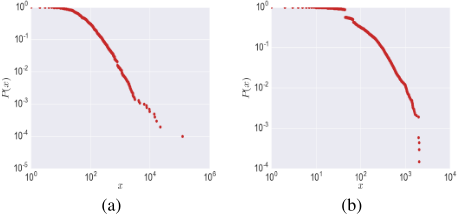
We test our model on several large datasets from Amazon.com [McAuley and Leskovec, 2013]. The datasets contain a variety of categories ranging from Shoes to Cellphones. Moreover, we crawled the price information of the products from a Amazon price tracking website 2 . The detailed statistics of the datasets are listed in Table 2. We are also interested in the diversities of users' total budgets. We plot the distributions of users' expenditures on products in the categories of Sports and Baby in Figure 2. The results show that few users spent much in online shopping while most of the users spent little. This phenomenon is in inline with the user activity levels [Gopalan et al., 2013].
| Variable | Type | Complement Conditional | Parameters | Relevant Expectations |
|---|---|---|---|---|
| θuk | Gamma | a + ∑v zbuik, πu+∑v βvk | ˜ θshp uk ,˜ θrte uk | a + ∑v yuv ˜ za uvk, ζ shp u ζrte u + ∑v ˜ βshp uk ˜ βrte uk |
| φuk | Gamma | e + ∑v za uik, ζu+∑v βvk | ˜ φshp uk , ˜ φrte uk | e + ∑v puv ˜ zbuvk, πshp u πrte u + ∑v ˜ βshp uk ˜ βrte |
| βuk | Gamma | c + ∑u za uvk + ∑u zbuvk , ηu+∑u θuk+∑u φuk | ˜ βshp uk , ˜ βrte uk | uk c + ∑u yuv ˜ za uvk + ∑u puv ˜ zbuvk, ηshp u ηrte u + ∑u ˜ θshp uk ˜ θrte uk + ∑u ˜ φshp uk ˜ φrte uk |
| ζu | Gamma | a′ +Ka, b′ + ∑k θuk | ˜ ζ shp uk ,˜ ζ rte uk | a + ∑v yuv ˜ za uvk, ζ shp u ζrte u + ∑v ˜ βshp uk ˜ βrte uk |
| ηv | Gamma | c′ +Kc, d′ + ∑k βuk | ˜ ηshp uk ,˜ ηrte uk | a + ∑v yuv ˜ za uvk, ζ shp u ζrte u + ∑v ˜ βshp uk ˜ βrte uk |
| πu | Gamma | e′ +Ke, f ′ + ∑k φuk | ˜πshp uk ,˜πrte uk | a + ∑v yuv ˜ za uvk, ζ shp u ζrte u + ∑v ˜ βshp uk ˜ βrte |
| za uv | Mult | log θuk + log βvk | ˜ za uv | uk exp{Ψ( ˜ θshp uk ) - log(˜ θrte uk ) +Ψ(˜ βshp uk ) - log(˜ βrte uk )} ˜ ˜ |
| zbuv | Mult | log φuk + log βvk | ˜ zbuv | exp{Ψ( φshp uk ) - log(˜ φrte uk ) + Ψ( βshp uk ) - log(˜ βrte uk )} |
| Shoes | Tools | Toys | Baby | Sports | Arts | Pet | Clothing | Cellphone | Patio | |
|---|---|---|---|---|---|---|---|---|---|---|
| Users | 12,421 | 4,566 | 8,869 | 7,057 | 14,124 | 1,815 | 2,035 | 14,560 | 1,485 | 2,700 |
| Items | 3,278 | 2,668 | 12,512 | 1,320 | 5,658 | 1,057 | 1,486 | 3,139 | 1,120 | 1,484 |
| Observations | 60,974 | 15,995 | 18,607 | 18,607 | 25,705 | 4,073 | 4,941 | 49,890 | 4,530 | 4,607 |
| Average spending ($) | 416.30 | 11,985.25 | 243.94 | 129.69 | 122.83 | 71.60 | 61.26 | 68.72 | 170.26 | 183.83 |
| Average rating | 4.36 | 4.21 | 4.27 | 4.00 | 4.29 | 4.28 | 4.12 | 4.23 | 3.74 | 4.06 |
We further normalize the prices to be compatible with the range of the ratings. We denote the maximum and minimum price of a specific category as pmax and pmin separately. And the maximum rating is denoted as L, which is usually 5. We then translate a specific price p using L p-pmin pmax-pmin and round the result to the nearest integer.
2 www.camelcamelcamel.com
6.2 Baselines
We compare our model with several state-of-the-art budgetunaware recommendation models.
HPF: Hierarchical Poisson factorization (HPF) [Gopalan et al., 2013] is the state-of-the-art collaborative filtering recommendation model. It only considers users' ratings. We adopt the implementation of HPF by the original authors.
BPR: Bayesian personalized ranking (BPR) [Rendle et al., 2009] is the state-of-the-art pairwise recommendation model for implicit feedback.We view ratings below 3 as positive feedback and implement BPR as described in [Rendle et al., 2009].
CliMF: CliMF [Shi et al., 2012] is the state-of-the-art ranking model for optimizing mean reciprocal rank. We use the implementation of CliMF of Graphchi [Kyrola et al., 2012].
PopRank: This is a naive baseline which considers recommending the users with the most popular items in the training set.
6.3 Parameter Settings and Evaluations
Similar to the settings of [Gopalan et al., 2013], we split each dataset into three parts: 70% of the dataset is served as training set, 20% of the dataset is served as test set and the remaining 10% is served as validation set. All the hyperparameters are tuned to work the best on the validation set. For CBPF and HPF, we set each Gamma shape and rate hyperparameter to 0.3. For BPR, the learning rate is 0.001 and the regularization parameter is 0.5. For CliMF, the learning rate is 0.005 and the regularization parameter is 0.01. And we fix the dimension of the latent vectors of all models to 10 for fair comparison.
| Shoes | Tools | Toys | Baby | Sports | Arts | Pet | Clothing | Cellphones | Patio | |
|---|---|---|---|---|---|---|---|---|---|---|
| CBPF | 0.12203 | 0.01614 | 0.05612 | 0.02930 | 0.03476 | 0.04653 | 0.01952 | 0.09549 | 0.02335 | 0.03364 |
| HPF | 0.11750 | 0.01508 | 0.04782 | 0.02457 | 0.03416 | 0.04365 | 0.01727 | 0.08509 | 0.02081 | 0.03225 |
| BPR | 0.10968 | 0.00801 | 0.01629 | 0.02229 | 0.01075 | 0.04790 | 0.01556 | 0.01535 | 0.02284 | .0.02469 |
| CliMF | 0.02515 | 0.00396 | 0.00461 | 0.02707 | 0.01197 | 0.01942 | 0.01209 | 0.01124 | 0.01838 | 0.01926 |
| PopRank | 0.00150 | 0.00362 | 0.00475 | 0.02733 | 0.00886 | 0.01813 | 0.01266 | 0.01189 | 0.02017 | 0.01802 |
| Shoes | Tools | Toys | Baby | Sports | Arts | Pet | Clothing | Cellphones | Patio | |
|---|---|---|---|---|---|---|---|---|---|---|
| CBPF | 0.32247 | 0.11307 | 0.09571 | 0.16953 | 0.08610 | 0.13842 | 0.04145 | 0.21608 | 0.15588 | 0.16473 |
| HPF | 0.30376 | 0.10845 | 0.08603 | 0.15072 | 0.07968 | 0.11528 | 0.03265 | 0.20645 | 0.15271 | 0.15964 |
| BPR | 0.02342 | 0.01345 | 0.02105 | 0.08304 | 0.01980 | 0.06993 | 0.03113 | 0.05042 | 0.03766 | 0.03852 |
| CliMF | 0.03102 | 0.03526 | 0.00729 | 0.04257 | 0.02823 | 0.07507 | 0.03061 | 0.04464 | 0.14778 | 0.14759 |
| PopRank | 0.00269 | 0.01828 | 0.00573 | 0.04919 | 0.00984 | 0.03470 | 0.02741 | 0.02118 | 0.04348 | 0.03081 |

In each round, we compute the average predictive loglikelihood of the validation set, the convergence of CBPF is guaranteed when the change of the log-likelihood is less than 0.001%. After fitting the model in the training set, for a specific user u, we calculate the ranking score fu(v) for each item v in the test set. The items with higher ranking scores are ranked higher in the recommended list. We adopt precisionat-K, recall-at-K and normalized cumulative reciprocal rank (NCRR) [Chaney et al., 2015] to measure the ranking performance of the models.
6.4 Results Analysis
We show the results of precision-at-10 and NCRR of all models in Table 3 and Table 4. Best performance is in bold font. And the results of recall-at-K (K ∈ {10,20,30,40,50}) are shown in Figure 4. As we can see, CBPF nearly beats all the baselines across all the categories. In most of the categories the improvements are significant. Moreover, our model exhibits particularly obvious improvements over some cold start categories where users have few ratings. The average improvement of precision-at-10 is 9.72%. The results empirically prove the importance of modeling users' budgets for recommendation. By finding what attributes the users will assign more budgets and avoiding recommending users with inappropriately expensive or cheap products, we can form more reasonable and more accurate recommendation results. The performance of BPR and CliMF is consistently lower than CBPF and HPF. One plausible reason is that their optimization goal is not directly related to the ranking metrics we compare here. We also examine the parameter sensitivity of CBPF. The results show that our model is rather stable with respect to the change of hyperparameters.
7 Conclusion
In this paper, we propose an original generative model named collaborative budget-aware Poisson factorization (CBPF) to connect users' ratings and budgets in a natural and cohesive manner. The model enjoys high interpretability and emphasizes the significance of modeling users' budgets. Extensive experimental results empirically prove the rationality and importance of the proposed model. We hope that the proposed model will prove useful for online shopping websites. Future works include considering modeling users' ratings and budgets in a dynamic and sequential manner.
Acknowledgments
This research is supported by the National Natural Science Foundation of China (NSFC) No.61672449 and No.61472347.
@inproceedings{ijcai2017p247,
  title     = {Understanding Users' Budgets for Recommendation with Hierarchical Poisson Factorization},
  author    = {Guo, Yunhui and Xu, Congfu and Song, Hanzhang and Wang, Xin},
  booktitle = {Proceedings of the Twenty-Sixth International Joint Conference on
               Artificial Intelligence, {IJCAI-17}},
  publisher = {International Joint Conferences on Artificial Intelligence Organization},
  editor    = {Carles Sierra},
  pages     = {1781--1787},
  year      = {2017},
  month     = {8},
  note      = {Main track},
  doi       = {10.24963/ijcai.2017/247},
  url       = {https://doi.org/10.24963/ijcai.2017/247},
}
TY - CPAPER TI - Understanding Users' Budgets for Recommendation with Hierarchical Poisson Factorization AU - Guo, Yunhui AU - Xu, Congfu AU - Song, Hanzhang AU - Wang, Xin T2 - Proceedings of the Twenty-Sixth International Joint Conference on Artificial Intelligence, IJCAI-17 PB - International Joint Conferences on Artificial Intelligence Organization PY - 2017 SP - 1781 EP - 1787 DO - 10.24963/ijcai.2017/247 UR - https://doi.org/10.24963/ijcai.2017/247 ER -Copied
Machine-readable versions of this paper, for tools and AI agents:





