
Exclusivity Regularized Machine: A New Ensemble SVM Classifier
Proceedings of the Twenty-Sixth International Joint Conference on Artificial Intelligence. Main track. Pages 1739-1745.
https://doi.org/10.24963/ijcai.2017/241
Keywords
- Machine Learning: Ensemble Methods
- Machine Learning: Classification
Abstract
The diversity of base learners is of utmost importance to a good ensemble. This paper defines a novel measurement of diversity, termed as exclusivity. With the designed exclusivity, we further propose an ensemble SVM classifier, namely Exclusivity Regularized Machine (ExRM), to jointly suppress the training error of ensemble and enhance the diversity between bases. Moreover, an Augmented Lagrange Multiplier based algorithm is customized to effectively and efficiently seek the optimal solution of ExRM. Theoretical analysis on convergence, global optimality and linear complexity of the proposed algorithm, as well as experiments are provided to reveal the efficacy of our method and show its superiority over state-of-the-arts in terms of accuracy and efficiency.
- [Altman, 1992] N. Altman. An introduction to kernel and nearest-neighbor nonparametric regression. The American Statistician, 46(3):175-185, 1992.
- [Breiman et al., 1984] L. Breiman, J. Friedman, R. Olshen, and C. Stone. Classification and Regression Trees. Wadsworth, Belmont, 1984.
- [Breiman, 1996] L. Breiman. Bagging predictors. Machine Learning, 24(2):123-140, 1996.
- [Breiman, 2001] L. Breiman. Random forests. Machine Learning, 45(1):5-32, 2001.
- [Chang et al., 2008] K. Chang, C. Hsieh, and C. Lin. Coor- dinate descent method for large-scale L 2 -loss linear svm. Journal of Machine Learning Research, 9:1369-1398, 2008.
- [Dietterich, 2000] T. Dietterich. An experimental compari- son of three methods for constructing ensembles of deci- sion trees: Bagging, boosting, and randomization. Ma- chine Learning, 40(2):139-157, 2000.
- [Domingos and Pazzani, 1997] P. Domingos and M. Paz- zani. On the optimality of the simple bayesian classifi- er under zero-one loss. Machine Learning, 29:103-130, 1997.
- [Du and Ling, 2014] L. Du and H. Ling. Exploiting compe- tition relationship for robust visual recognition. In AAAI, pages 2746-2752, 2014.
- [Fisher, 1936] R. Fisher. The use of multiple measurements in taxonomic problems. Annals of Eugenics, 7(2):179- 188, 1936.
- [Freund and Schapire, 1997] Y. Freund and R. Schapire. A decision-theoretic generalization of on-line learning and an application to boosting. Journal of Computer and Sys- tem Sciences, 55(1):119-139, 1997.
- [Giacinto and Roli, 2001] G. Giacinto and F. Roli. Design of effective neural network ensembles for image classi- fication purposes. Image and Vision Computing, 19(9- 10):699-707, 2001.
- [Ho, 1998] T. Ho. The random subspace method for con- structing decision forests. IEEE Transactions on Pattern Analysis and Machine Intelligence, 20(8):832-844, 1998.
- [Hsieh et al., 2008] C. Hsieh, K. Chang, S. Keerthi, S. Sun- dararajan, and C. Lin. A dual coordinate descent method for large-scale linear svm. In ICML, pages 408-415, 2008.
- [Joachims, 2006] T. Joachims. Training linear svms in linear time. In ACM SIGKDD, pages 217-226, 2006.
- [Keerthi and DeCoste, 2005] S. Keerthi and D. DeCoste. A modified finite newton method for fast solution of large scale linear svms. Journal of Machine Learning Research, 6:627-650, 2005.
- [Kong et al., 2014] D. Kong, R. Fujimaki, J. Liu, F. Nie, and C. Ding. Exclusive feature learning on arbitrary structures via ℓ 1,2 -norm. In NIPS, pages 1655-1663, 2014.
- [Kowalski, 2009] M. Kowalski. Sparse regression using mixed norms. Applied and Computational Harmonic Analysis, 27(3):303-324, 2009.
- [Krogh and Vedelsby, 1995] A. Krogh and J. Vedelsby. Neu- ral network ensembles, cross validation, and active learn- ing. In NIPS, pages 231-238, 1995.
- [Kuncheva et al., 2003] L. Kuncheva, C. Whitaker, C. Ship- p, and R. Duin. Limits on the majority vote accuracy in classification fusion. Pattern Analysis and Applications, 6(1):22-31, 2003.
- [Li et al., 2012] N. Li, Y. Yu, and Z. Zhou. Diversity regular- ized ensemble pruning. In ECML PKDD, pages 330-345, 2012.
- [Lin et al., 2008] C. Lin, R. Weng, and S. Keerthi. Trust region newton method for large-scale logistic regression. Journal of Machine Learning Research, 9:627-650, 2008.
- [Nie et al., 2014] F. Nie, Y. Huang, X. Wang, and H. Huang. New primal svm solver with linear computational cost for big data classifications. In ICML, Beijing, China, 2014.
- [Quinlan, 1993] J. Quinlan. C4.5: Programs for machine learning. Morgan Kaufmann Publisher, San Mateo, 1993.
- [Rodriguez et al., 2006] J. Rodriguez, L. Kubcheva, and C. Alonso. Rotation forest: A new classifier ensemble method. TPAMI, 28(10):1619-1630, 2006.
- [Shalev-Shwartz et al., 2007] S. Shalev-Shwartz, Y. Singer, and N. Srebro. Pegasos: Primal estimated subgradient solver for svm. In ICML, pages 807-814, 2007.
- [Teo et al., 2010] C. Teo, S. Vishwanathan, A. Smola, and Q. Le. Bundle methods for regularized risk minimiza- tion. Journal of Machine Learning Research, 11:311-365, 2010.
- [Ueda and Nakano, 1996] P. Ueda and R. Nakano. General- ization error of ensemble estimators. In Proceedings of In- ternational Conference on Neural Network (ICNN), pages 90-95, 1996.
- [Vapnik, 1995] V. Vapnik. The Nature of Statistical Learning Theory. Springe-Verlag, New York, NY, 1995.
- [Xie et al., 2015a] P. Xie, Y. Deng, and E. Xing. Latent vari- able modeling with diversity-inducing mutual angular reg- ularization. arXiv:1512.07336v1, 2015.
- [Xie et al., 2015b] P. Xie, Y. Deng, and E. Xing. On the generalization error bounds of neural networks under diversity-inducing mutual angular regularization. arX- iv:1511.07110v1, 2015.
- [Yu et al., 2011] Y. Yu, Y. Li, and Z. Zhou. Diversity regu- larized machine. In IJCAI, pages 1603-1608, 2011. IJCAI
- [Zhang et al., 2010] Y. Zhang, R. Jin, and S. Hoi. Exclusive lasso for multi-task feature selection. In AISTATS, pages 988-995, 2010.
- [Zhou, 2012] Z. Zhou. Ensemble Methods: Foundations and Algorithms. Taylor & Francis Group, LLC, Boca Raton, FL, 2012.
References were extracted automatically from the PDF and may contain errors.
Full text extracted automatically from the PDF; figures, tables and equations may differ. The PDF is the version of record.
1 Introduction
Classification is a major task in machine learning and pattern recognition. In binary classification, a hypothesis is constructed from a feasible hypothesis space based on the training set {(xi, yi)}Ni=1 , where {xi}Ni=1 is a set of data points with xi ∈ Rd sampled i.i.d. under a distribution from an input subspace, and {yi}Ni=1 with yi ∈ {-1,+1} is the corresponding label set. The obtained hypothesis, also known as classifier, is "good" when it is capable to generalize well the "knowledge" learned from the training data to unseen instances. Multi-class cases can be analogously accomplished by a group of binary classifiers.
Over the past decades, numerous classifiers have been devised. The k-nearest neighbor (k-NN) [Altman, 1992] is an intuitive and simple one. However, its performance heavily depends on the selection of k and is sensitive to noisy data, making k-NN vulnerable in practice. Decision tree (DT) learning is to construct a tree by partitioning the source set into subsets according to a feature test. CART [Breiman et al., 1984] and C4.5 [Quinlan, 1993] are two examples of DT. The main drawbacks of decision trees are their sub-optimality and overfitting problems. Support vector machine (SVM) [Vapnik, 1995], as one of the most robust and accurate approaches, aims to find a hyperplane with the maximum margin between classes. Besides, linear discriminant analysis [Fisher,
1936] and naive Bayes [Domingos and Pazzani, 1997] are other classic classifiers.
As has been well recognized, a combination of various classifiers can improve predictions. Ensemble approaches, with Boosting [Freund and Schapire, 1997] and Bagging [Breiman, 1996] as representatives, make use of this recognition and achieve strong generalization performance [Zhou, 2012]. The generalization error of ensemble mainly depends on two factors, formally expressed as E = ¯E - ¯ A, where E is the mean-square error of the ensemble, ¯E represents the average mean-square error of component learners and ¯ A stands for the average squared difference (diversity) between the ensemble and the components. Error-Ambiguity decomposition [Krogh and Vedelsby, 1995], Bias-VarianceCovariance decomposition [Ueda and Nakano, 1996] and Strength-Correlation decomposition [Breiman, 2001] all confirm the above principle. Specifically, Boosting is a family of ensemble learning meta-algorithms, which improves the classification performance through letting the subsequent base learner pay more attention on data that have been wrongly grouped by the previous bases. AdaBoost is probably the most prominent Boosting scheme. While Bagging represents another category that tries to train a set of diverse weak classifiers by utilizing the bootstrap sampling technique. Several specific algorithms, such as random subspace [Ho, 1998], random forest [Breiman, 2001] and rotation forest [Rodriguez et al., 2006], have been proposed to further enforce the diversity of ensemble members. Certainly, both Boosting and Bagging can be applied to (most of) the conventional classifiers, e.g. DT and SVM.
Considering the popularity of SVM and the potential of ensemble, it would be beneficial to equip SVM with ensemble thoughts. Employing SVM as the base learner of Bagging or Boosting is a natural manner. Alternatively, this work provides a model to train a set of SVMs and integrate them as a homogeneous ensemble. The model jointly minimizes the training error and maximizes the diversity of base learners. Different from Bagging, our method does not rely on sampling schemes to achieve the diversity, although it is flexible to embrace such schemes. Additionally, the proposed method simultaneously trains all the base learners unlike Boosting methods doing the job sequentially. Concretely, the contribution of this paper can be summarized as follows: 1) we define a new measurement, namely (relaxed) exclusivity, to manage the diversity between base learners, 2) we propose a novel ensemble, called Exclusivity Regularized Machine (ExRM), which concerns the training error and the diversity of components simultaneously, and 3) we design an Augmented Lagrange Multiplier based algorithm to efficiently seek the solution of ExRM. Theoretical analysis on convergence, global optimality and linear complexity of the proposed algorithm is also provided.
2 Our Method
2.1 Preliminary
Arguably, SVM [Vapnik, 1995][Keerthi and DeCoste, 2005] is one of the most popular classifiers due to its promising performance. In general, the primal SVM (PSVM) can be modeled as follows:
where f(·) is a penalty function, Ψ(w) performs as a regularizer on the learner w and b is the bias. The function φ(·) is to map xi from the original D-dimensional feature space to a newM-dimensional one. Moreover, λ is a non-negative coefficient that provides a trade-off between the loss term and the regularizer. If PSVM adopts the hinge loss as penalty, the above (1) turns out to be:
where the operator (u)+ := max(u, 0) keeps the input scalar u unchanged if u is non-negative, returns zero otherwise, the extension of which to vectors and matrices is simply applied element-wise. Furthermore, p is a constant typically in the range [1, 2] for being meaningful. In practice, p is often selected to be either 1 or 2 for ease of computation, which correspond to ℓ1 -norm and ℓ2 -norm loss PSVMs, respectively. As for the regularization term, Ψ(w) := 1 2 ‖w‖22 (ℓ2 regularizer) and Ψ(w) := ‖w‖1 (ℓ1 regularizer) are two classical options.
2.2 Exclusivity RegularizedMachine
It is natural to extend the traditional PSVM (2) to the following ensemble version with C components as:
where W ∈ RM×C := [w1,w2, ...,wC] and b ∈ RC := [b1, b2, .., bC]T . Suppose we simply impose 12 ‖W‖2F or ‖W‖1 on W, all the components (and the ensemble) will have no difference with the hypothesis directly calculated from (2) using the same type of regularizer. 1 From this view, Ψ(W) is critical to achieving the diversity.
1 We note that splitting the training data into C sub-sets, like the bootstrap sampling, and training C classifiers separately on the subsets would lead to some difference between the components. However, this strategy does not essentially advocate the diversity of base learners. Although how to sample training subsets is not the focus of this work, our model has no difficulties to adopt such sampling strategies.
Prior to introducing our designed regularizer, we first focus on the concept of diversity. Although the diversity has no formal definition so far, the thing in common among studied measurements is that the diversity enforced in a pairwise form between members strikes a good balance between complexity and effectiveness. The evidence includes Q-statistics measure [Kuncheva et al., 2003], correlation coefficient measure [Kuncheva et al., 2003], disagreement measure [Ho, 1998], double-fault measure [Giacinto and Roli, 2001], k-statistic measure [Dietterich, 2000], mutual angular measure [Yu et al., 2011; Xie et al., 2015b; 2015a] and competition measure [Du and Ling, 2014]. These measures somehow enhance the diversity, however, most of them are heuristic. One exception is Diversity Regularized Machine [Yu et al., 2011], which attempts to seek the globally-optimal solution. Unfortunately, it often fails because the condition required for the global optimality, say ‖wc‖2 = 1 for all c, is not always satisfied. Further, Li et al. proposed a pruning scheme to improve the performance of DRM [Li et al., 2012]. But, DRM requires too much time to converge, which limits its applicability. Below, we define a new measure of diversity, i.e. (relaxed) exclusivity.
Definition 1. (Exclusivity) Exclusivity between two vectors u ∈ Rm and v ∈ Rm is defined as X (u, v) := ‖u ⊙ v‖0 = ∑mi=1 u(i) · v(i) ̸= 0, where ⊙ designates the Hadamard product, and ‖ · ‖0 is the ℓ0 norm.
From the definition, we can observe that the exclusivity encourages two vectors to be as orthogonal as possible. Due to the non-convexity and discontinuity of ℓ0 norm, we have the following relaxed exclusivity.
Definition 2. (Relaxed Exclusivity) The definition of relaxed exclusivity between u ∈ Rm and v ∈ Rm is given as Xr(u, v) := ‖u ⊙ v‖1 = ∑mi=1 |u(i)| · |v(i)|, where |u| is the absolute value of u. The relaxation is similar with that of the ℓ1 norm to the ℓ0 norm.
It can be easily verified that ‖u‖0 = X(u, 1), ‖u‖1 = Xr(u, 1) and ‖u‖22 = Xr(u, u), where 1 ∈ Rm is the vector with all of its m entries being 1.
Instead of directly employing ∑1≤˜ c̸=c≤C Xr(wc, w˜ c) as the final Ψ(W), we adopt the following:
The main reasons of bringing 12 ‖W‖2F into the regularizer are: 1) it essentially enhances the stability of solution, 2) it tends to mitigate the scale issue by penalizing large columns, and 3) as the relaxed exclusivity itself is non-convex, the introduction guarantees the convexity of the regularizer. Finally, the proposed Exclusivity Regularized Machine (ExRM) can be written in the following shape:
Remarks As expressed in Eq. (4), we have motivated the ℓ1,2 regularizer from a novel perspective. It has been verified that, as one of mixed norms, the ℓ1,2 is in nature able to capture some structured sparsity [Kowalski, 2009]. In general, the regression models using such mixed norms can be solved by a modified FOCUSS algorithm [Kowalski, 2009]. Zhou et al. [Zhang et al., 2010] introduced the ℓ1,2 regularizer into a specific task, i.e. multi-task feature selection, and used the subgradient method to seek the solution of the associated optimization problem. The responsibility of the ℓ1,2 regularizer is to enforce the negative correlation among categories [Zhang et al., 2010]. Recently, Kong et al. [Kong et al., 2014] utilized ℓ1,2 norm to bring out sparsity at intra-group level in feature selection, and proposed an effective iteratively re-weighted algorithm to solve the corresponding optimization problem. In this work, besides the view of motivating the ℓ1,2 regularizer, its role in our target problem, say constructing an ensemble of SVMs, is also different with the previous work [Kowalski, 2009; Zhang et al., 2010; Kong et al., 2014]. The functionalities of [Zhang et al., 2010] and [Kong et al., 2014] are the intra-exclusivity of multiple hypotheses (tasks) and the inter-exclusivity of a single hypothesis respectively, while our principle is the diversity of multiple components of a single ensemble hypothesis.
2.3 Optimization
With the trick that 1 - (φ(xi)T wc + bc)yi = yiyi - (φ(xi)T wc + bc)yi = yi(yi - (φ(xi)T wc + bc)), we introduce auxiliary variables eci := yi - (φ(xi)T wc + bc). In the sequel, the minimization of (5) can be converted into:
where X ∈ RM×N := [φ(x1), φ(x2), ..., φ(xN)], ec ∈ RN := [ec1 , ec2 , ..., ecN ]T , E ∈ RN×C := [e1 , e2 , ..., eC ] and y ∈ RN := [y1, y2, ..., yN]T . And each column of Y ∈ RN×C is y. Please note that, the constraint P = W is added to make the objective separable and thus solvable by the ALM framework. It is worth mentioning that, thanks to the convexity of each term in the objective and the linearity of the constraints, the target problem is convex. The Lagrangian function of (6) can be written in the following form:
with the definition Φ(U,V) := µ2 ‖V‖2F + 〈U,V〉, where 〈·, ·〉 represents matrix inner product and µ is a positive penalty scalar. In addition, Q ∈ RM×C and Z ∈ RN×C are Lagrangian multipliers. The proposed solver iteratively updates one variable at a time by fixing the others. Below are the solutions to sub-problems.
W sub-problem With the variables unrelated to W fixed, we have the sub-problem of W:
As observed from the problem (8), it can be split into a set of smaller problems. For each rowW·j, instead of directly optimizing (8), we resolve the following equivalent objective:
where G is formed by:
where ϵ → 0+ (a small constant) is introduced to avoid zero denominators. 2 Since both G and W·j depend on W·j, to find out the solution to (9), we employ an efficient reweighted algorithm to iteratively update G and W·j . As for W·j , with G fixed, equating the partial derivative of (9) with respect toW·j to zero yields:
Then G(k+1) is updated using W(k+1) ·j as in (10). The procedure summarized in Alg. 1 terminates when converged. b sub-problem Dropping the terms independent on b leads to a least squares regression problem:
E sub-problem Similarly, picking out the terms related to E gives the following problem:
where S(t) :=Y-XT P(t) -1b(t+1)T - Z(t) µ(t) . It can be seen that the above is a single-variable 2-piece piecewise function. Thus, to seek the minimum of each element in E, we just need to pick the smaller between the minima when yieci ≥ 0 and yieci < 0. Moreover, we can provide the explicit solution when p := 1 or 2 (for arbitrary p we will discuss it latter). When p := 1:
For p := 2:
where Ω ∈ RN×C := (Y ◦ S(t) > 0) is an indicator matrix, and ¯Ω is the complementary support of Ω. The definition of shrinkage operator on scalars is Sϵ>0[u] := sgn(u) max(|u| - ϵ, 0). The extension of the shrinkage operator to vectors and matrices is simply applied element-wise.
2 The derived algorithm can be proved to minimize ‖WT +ϵ‖21,2. Certainly, when ϵ → 0+, ‖WT + ϵ‖21,2 infinitely approaches to ‖WT ‖21,2.
Algorithm 1: W Solver
Input: W(t) , P(t) , Q(t) , µ(t) . Initial.: k ← 0; H(k) ←W(t) ; for j = 0 : M do while not converged do Update G(k+1) via Eq. (10); Update H(k+1) ·j via Eq. (11); k ← k +1; end end Output: W(t+1) ← H(k)Algorithm 2: Exclusivity Regularized Machine
Input: Training set {(xi, yi)}Ni=1 , positive integer C and
P sub-problem There are two terms involving P. The associated optimization problem reads:
Its closed-form solution can be obtained by:
where we denote K := (I + XXT )-1 and M := Y - 1b(t+1)T - Z(t) µ(t) .
Multipliers and µ Two multipliers and µ are updated by:
For clarity, the procedure of solving (2) is outlined in Algorithm 2. The algorithm should not be terminated until the change of objective value is smaller than a pre-defined threshold (in the experiments, we use 0.05). Please see Algorithm 2 for other details that we can not cover in the text.
3 Theoretical Analysis
First, we come to the loss term of ExRM (5), which assesses the total penalty of base learners as ∑Cc=1 ∑Ni=1 (1 - (φ(xi)T wc + bc)yi )p+, where p ≥ 1. Alternatively, the loss of the ensemble {we, be} := { 1C ∑Cc=1 wc, 1C ∑Cc=1 bc} is ∑Ni=1 (1 - (φ(xi)T we + be)yi )p+. We have the relationship between the two losses as described in Proposition 1.
Proposition 1. Let {w1, b1},..., {wC, bC} be the component learners obtained by ExRM (Alg. 2), and {we, be} := { 1C ∑Cc=1 wc, 1C ∑Cc=1 bc} the ensemble, the loss of {we, be} is bounded by the average loss of the base learners.
Proof. This can be established by Jensen's inequality.
The proposition indicates that as we optimize ExRM (5), an upper bound of the loss of the ensemble is also minimized. Thus, incorporating with our proposed regularizer, ExRM is able to achieve the goal of simultaneously optimizing the training error of ensemble and the diversity of components.
One may wonder why not minimizing the loss of the ensemble, which seems reasonable, like:
The reason is that the optimal solution of (19) is exactly that of PSVM (2). The solution of (19) satisfies that one entry in the i-th row of W is we(i) and the rest ones are all zero, having the columns of W absolutely independent. But, the exclusivity achieved in this way is meaningless. According to Proposition 1, their equivalence is reached when each wc is identical with we. Based on the analysis above, we can say that, compared with (19), ExRM is more proper, which desires to find a balance between the diversity and consistency (training error) of base learners.
Next, we shall consider the convergence and optimality of the designed algorithms. We first confirm the property of Alg. 1, which is established by Theorem 1.
Theorem 1. The updating rules (10) and (11) for solving the problem (9), i.e. Algorithm 1, converges and the obtained optimal solution is exactly the global optimal solution of the problem (8).
Proof. Algorithm 1 is actually a special case of the algorithm proposed in [Kong et al., 2014]. We refer readers to [Kong et al., 2014] for the detailed proof.
With Theorem 1, we have come to the convergence and optimality of our proposed Algorithm 2.
Theorem 2. The solution consisting of the limit of the sequences {W(t) }, {b(t) } and {E(t) } generated by Algorithm 2, i.e. (W(∞) , b(∞) ,E(∞) ), is global optimal to ExRM (5), and the convergence rate is at least o( 1 µ(t) ).
Proof. Due to space limit, instead of the complete proof, we here only provide the proof sketch including three main steps: 1) (W(t) , b(t) ,E(t) ) approaches to a feasible solution, i.e. limt→∞‖P(t) - W(t) ‖F = 0 and limt→∞‖E(t) - Y + XtP(t) + 1b(t)T ‖F = 0; 2) All of
{P(t) }, {Z(t) }, {Q(t) }, {W(t) }, {b(t) } and {E(t) } are bounded; 3) limt→∞ 12 ‖W(t) ‖21,2 + λ‖(Y ◦ E(t) )+‖pp = limt→∞ Lμ(t-1) (W(t) , b(t) , E(t) , P(t) , Q(t-1) , Z(t-1) ) due to Lμ(t-1)(W(t) , b(t) , E(t) , P(t) , Q(t-1) , Z(t-1) ) = 12 ‖W(t) ‖21,2 + λ‖(Y ◦ E(t) )+‖pp + ‖Q(t) ‖2F -‖Q(t-1) ‖2F 2μ(t-1) + ‖Z(t) ‖2F -‖Z(t-1) ‖2F 2μ(t-1) . Then the conclusion can be drawn with the feasibility of solution by Alg. 2, the convexity of problem (5), and the (descending) property of an ALM algorithm.
In addition, we show the complexity of Alg. 2. Updating each row of W takes O(qC 2 ) and O(qC) for (11) and (10) respectively, where q is the (inner) iteration number of Alg. 1. Please note that, due to the diagonality of G, the inverse of G + μI only needs O(C). Therefore, the cost of Alg. 1 is O(qC 2M ). The b sub-problem requires O(CMN ). The complexity of the E sub-problem is O(CMN ), for both p := 1 and p := 2. Solving P spends O(CMN + CM 2 ). Besides, the update of the multipliers is at O(CMN ) expense. In summary, Alg. 2 has the complexity of O(tCM (qC + N + M )), where t is the number of (outer) iterations required to converge.
4 Experimental Verification
We adopt several popular UCI benchmark datasets for performance evaluation. 3 All experiments are conducted on a machine with 2.5 GHz CPU and 64G RAM.
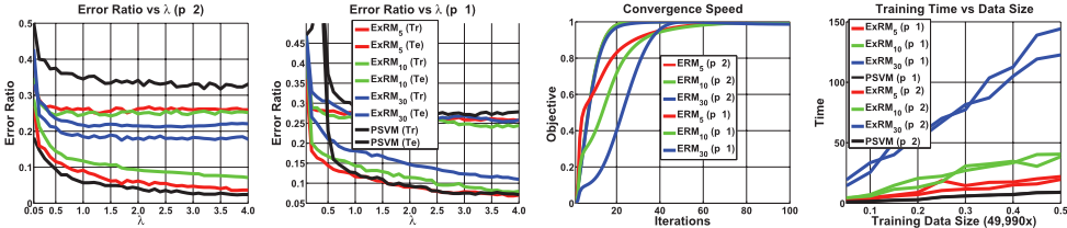
Parameter Effect Here, we evaluate the training and testing errors of ExRMC (C ∈ {5, 10, 30} means the component number) against varying values of λ in the range [0.05, 4]. All the results shown in this experiment are averaged over 10 independent trials, each of which randomly samples half data from the sonar dataset for training and the other half for testing. The first picture in Fig. 1 displays the training error and testing error plots of L2 loss ExRM with L2 loss PSVM [Nie et al., 2014] (denoted as L2-PSVM) as reference. From the curves, we can observe that, as λ grows, the training errors drop, as well as composing less base learners leads to a smaller training error. This is because more and more effort is put on fitting data. As regards the testing error, the order is reversed, which corroborates the recognition that the predication gains from the diversity of classifiers, and reveals the effectiveness of our design in comparison with L2-PSVM. Besides, the testing errors change very slightly in a relatively large range of λ, which implies the insensitivity of ExRM to λ. The second picture corresponding to p := 1 shows an additional evidence to p := 2. Although the performance gaps between the different cases shrink, the improvement of ExRM is still noticeable. Based on this evaluation, we set λ to 2 for both L1-ExRM and L2-ExRM in the rest experiments.
3 Available at www.csie.ntu.edu.tw/∼cjlin/libsvmtools/datasets
Convergence Speed & Training Time Although the convergence rate and complexity of the proposed algorithm have been theoretically provided, it would be more intuitive to see its empirical behavior. Thus, we here show how quick the algorithm converges, without loss of generality, on the ijcnn1 dataset. From the third picture in Fig. 1, we can observe that, when p := 2, all the three cases converge with about 30 iterations. The cases correspond to p := 1 take more iterations than p := 2 (about 70 iterations), but they are still very efficient. Please note that, for a better view of different settings, the objective plots are normalized into the range [0, 1]. The rightmost picture in Fig. 1 gives curves of how the CPUtime used for training increases with respect to the number of training samples. Since the training time is too short to be accurately recorded, we carry out each test for 10 independent trials, and report the total training time (in seconds). As can be seen, the training time for both p := 1 and 2 is quasi linear with respect to the size of training data. For all the three cases that correspond to ExRM5, ExRM10 and ExRM30, the choice of p barely brings differences in time. The gaps between the three cases dominantly come from the number of base learners. The PSVM only needs to learn one classifier while ExRM requires to train multiple bases. 4
Performance Comparison This part first compares our proposed ExRM with the classic ensemble models including AdaBoost and Bagging with Tree as the base learner (denoted as AdaTree and BagTree, respectively), and the recently designed DRM. The codes of DRM are downloaded from the authors' website, while those of AdaTree and BagTree are integrated in the Matlab statistics toolbox (fitensemble). The base of DRM, ν-SVM, is from LibSVM.
Table 1 provides the quantitative comparison among the competitors. We report the mean testing errors over 10 independent trials. Since the sizes and distributions of the datasets vary, to avoid the effect brought by the amount of training data and test the generalization ability of the ensembles learned from different types of data, we randomly sample 150 data points from a dataset as its training set and the rest as the testing. AdaTree and BagTree are inferior to ExRM and DRM in most cases. The exception is on the splice dataset. As for our ExRM, we can see that it significantly outperforms the others on australian, sonar, heart and ionosphere, and competes very favorably on the german dataset. On each dataset, we assign ranks to methods. The average ranks (A.R.) of the competitors over the involved datasets are given in the last column of Tab. 1. It can be observed that the top five average ranks are all lower than 5.0, and four of which are from ExRM methods. The best and the second best belong to L2-ExRM30 (A.R.=2.5) and L2-ExRM10 (A.R.=3.4) respectively, while the fourth and fifth places are taken by L1ExRM10 (A.R.=4.8) and L1-ExRM30 (A.R.=4.9) respectively. The third goes to DRM10, the average rank of which is 4.6. The results on the ijcnn1 are not included in the table, as all the methods perform very closely to each other, which may lead to an unreliable rank.
4 In [Nie et al., 2014], the authors have revealed via extensive experiments, that PSVM (SVM-ALM) is much more efficient than SVMperf [Joachims, 2006], Pegasos [Shalev-Shwartz et al., 2007], BMRM [Teo et al., 2010], and TRON [Lin et al., 2008], PCD [Chang et al., 2008] and DCD [Hsieh et al., 2008].
| Method (R) | german | diabetes | australian | sonar | splice | liver | heart | ionosphere | A.R. |
|---|---|---|---|---|---|---|---|---|---|
| L1-ExRM10 | 26.08±1.21 (5) | 24.73±1.44 (4) | 14.59±0.84 (6) | 23.62±3.64 (4) | 26.53±1.66 (7) | 42.82±2.41 (6) | 17.17±1.25 (2) | 13.68±2.60 (4) | 4.8 |
| L2-ExRM10 | 26.00±1.16 (3) | 24.34±0.92 (1) | 14.13±0.40 (3) | 23.79±4.36 (5) | 26.75±2.26 (8) | 36.00±4.05 (1) | 17.83±1.81 (4) | 13.03±2.20 (2) | 3.4 |
| AdaTree10 | 30.51±1.38 (8) | 29.24±2.73 (7) | 48.39±1.91 (9) | 27.59±6.08 (10) | 14.86±3.03 (3) | 46.92±3.59 (10) | 47.83±3.25 (9) | 30.05±3.13 (8) | 8.0 |
| BagTree10 | 31.59±2.59 (9) | 30.63±3.38 (9) | 46.43±2.58 (7) | 25.00±8.26 (6) | 19.26±1.78 (4) | 46.00±3.58 (8) | 47.58±1.94 (7) | 38.71±3.02 (10) | 7.5 |
| DRM10 | 25.98±1.20 (2) | 24.47±0.89 (2) | 14.09±1.55 (2) | 27.07±3.05 (9) | 35.96±2.85 (9) | 36.77±3.79 (3) | 19.00±2.22 (5) | 19.50±3.67 (5) | 4.6 |
| L1-ExRM30 | 26.27±1.02 (6) | 33.50±1.92 (10) | 14.24±1.02 (4) | 23.62±2.82 (3) | 25.64±1.63 (5) | 42.77±2.48 (5) | 17.17±2.30 (3) | 13.30±2.17 (3) | 4.9 |
| L2-ExRM30 | 25.75±1.10 (1) | 25.42±1.41 (5) | 14.02±0.81 (1) | 21.55±3.66 (1) | 26.07±1.80 (6) | 40.05±3.48 (4) | 17.08±1.26 (1) | 12.99±1.95 (1) | 2.5 |
| AdaTree30 | 32.22±2.32 (10) | 29.85±2.77 (8) | 48.94±2.13 (10) | 25.17±7.63 (7) | 14.45±2.53 (2) | 46.26±3.97 (9) | 47.58±3.27 (8) | 32.34±3.25 (9) | 7.9 |
| BagTree30 | 29.16±1.02 (7) | 28.58±2.81(6) | 46.59±1.39 (8) | 21.72±4.24 (2) | 14.00±1.96 (1) | 45.85±2.23 (7) | 48.08±4.21 (10) | 27.86±2.27 (7) | 6.0 |
| DRM30 | 26.05±1.14 (4) | 24.47±0.89 (2) | 14.43±1.65 (5) | 26.55±3.91 (8) | 35.98±2.84 (10) | 36.67±4.03 (2) | 19.00±2.51 (6) | 19.70±3.48 (6) | 5.4 |
| L1-ExRM10 | L2-ExRM10 | AdaTree10 | BagTree10 | DRM10 | L1-ExRM30 | L2-ExRM30 | AdaTree30 | BagTree30 | DRM30 |
| 0.0568 | 0.0575 | 0.1758 | 0.3019 | 16.86 | 0.1358 | 0.1091 | 0.2841 | 0.2512 | 59.38 |
Another issue should be concerned is the efficiency. Table 2 lists the mean training time over all the datasets and each dataset executes 10 runs. From the numbers, we can see the clear advantage of our ExRM. L1-ExRM10 and L2-ExRM10 only spend about 0.05s on training, while the ExRMs with 30 components, i.e. L1-ExRM30 and L2-ExRM30, cost less than 0.14s. Both AdaTree and BagTree are sufficiently efficient, which take less than 0.3s to accomplish the task. But the training uses 16.86s and 59.38s by DRM for the 10-base and 30-base cases respectively. We would like to mention that the core of DRM is implemented in C++, while our ExRM is in pure Matlab. Moreover, as theoretically analyzed and empirically verified, our algorithm is linear with respect to the size of training set.
As aforementioned, employing SVM as the base of AdaBoost or Bagging is a way to construct an ensemble SVM. Here, we repeat the previous experiment to see the difference among AdaBoost plus L2-PSVM (AdaSVM), Bagging plus L2-PSVM (BagSVM), DRM and our L2-ExRM. Please note that L2-ExRM and DRM reduce to PSVM and ν-SVM respectively, when the base number is 1. Table 3 provides the average testing errors over all the datasets (each method runs 10 times). From the numbers, we can observe that both AdaSVM and BagSVM outperform DRM for all the cases, while ExRM shows the best results among the competitors.
| # Base | 1 | 5 | 10 | 30 |
|---|---|---|---|---|
| L1-ExRM | 26.30 (L1-PSVM) | 25.65 | 25.24 | 25.09 |
| L2-ExRM | 25.68 (L2-PSVM) | 24.80 | 24.41 | 24.85 |
| AdaSVM | - | 26.51 | 26.59 | 26.64 |
| BagSVM | - | 26.34 | 25.93 | 25.69 |
| DRM | 28.31(ν-SVM) | 27.85 | 27.70 | 27.89 |
5 Conclusion and Discussion
The diversity of component learners is critical to the ensemble performance. This paper has defined a new measurement of diversity, i.e. exclusivity. Incorporating the designed regularizer with the hinge loss function gives a birth to a novel model, namely ExRM. The convergence of the proposed ALM-based algorithm to a global optimal solution is theoretically guaranteed. ExRM can take into account more elaborate treatments for further improvement. For instance, thanks to the relationship ‖u‖1 = Xr(u, 1), the sparsity on W can be promoted by extending ˜W to [W, β1], where β is a weight coefficient of the sparsity. In addition, it is difficult to directly solve the E sub-problem (13) with arbitrary given p. Fortunately, in this work, it is always that p ≥ 1. Thus the partial derivative of (13) with respect to E is monotonically increasing. The binary search method can be employed to narrow the possible range of E by half via each operation. In this work, we did not take any advantages of Boosting and Bagging. It is positive that ExRM is able to act as the base learner for both Boosting and Bagging. By doing so, Boosting ExRM and Bagging ExRM can be viewed as ensembles of ensemble and expected to further boost the performance.
Acknowledgments
Xiaojie Guo is supported by National Natural Science Foundation of China (grant no. 61402467). Haibin Ling is supported by National Natural Science Foundation of China (grant no. 61528204) and National Science Foundation (grant no. 1350521).
@inproceedings{ijcai2017p241,
  title     = {Exclusivity Regularized Machine: A New Ensemble SVM Classifier},
  author    = {Guo, Xiaojie and Wang, Xiaobo and Ling, Haibin},
  booktitle = {Proceedings of the Twenty-Sixth International Joint Conference on
               Artificial Intelligence, {IJCAI-17}},
  publisher = {International Joint Conferences on Artificial Intelligence Organization},
  editor    = {Carles Sierra},
  pages     = {1739--1745},
  year      = {2017},
  month     = {8},
  note      = {Main track},
  doi       = {10.24963/ijcai.2017/241},
  url       = {https://doi.org/10.24963/ijcai.2017/241},
}
TY - CPAPER TI - Exclusivity Regularized Machine: A New Ensemble SVM Classifier AU - Guo, Xiaojie AU - Wang, Xiaobo AU - Ling, Haibin T2 - Proceedings of the Twenty-Sixth International Joint Conference on Artificial Intelligence, IJCAI-17 PB - International Joint Conferences on Artificial Intelligence Organization PY - 2017 SP - 1739 EP - 1745 DO - 10.24963/ijcai.2017/241 UR - https://doi.org/10.24963/ijcai.2017/241 ER -Copied
Machine-readable versions of this paper, for tools and AI agents:





