
Analogy-preserving functions: A way to extend Boolean samples
Proceedings of the Twenty-Sixth International Joint Conference on Artificial Intelligence. Main track. Pages 1575-1581.
https://doi.org/10.24963/ijcai.2017/218
Keywords
- Machine Learning: Machine Learning
- Machine Learning: New Problems
- Machine Learning: Classification
Abstract
Training set extension is an important issue in machine learning. Indeed when the examples at hand are in a limited quantity, the performances of standard classifiers may significantly decrease and it can be helpful to build additional examples. In this paper, we consider the use of analogical reasoning, and more particularly of analogical proportions for extending training sets. Here the ground truth labels are considered to be given by a (partially known) function. We examine the conditions that are required for such functions to ensure an error-free extension in a Boolean setting. To this end, we introduce the notion of Analogy Preserving (AP) functions, and we prove that their class is the class of affine Boolean functions. This noteworthy theoretical result is complemented with an empirical investigation of approximate AP functions, which suggests that they remain suitable for training set extension.
- [Bayoudh et al., 2007a] S. Bayoudh, L. Miclet, and A. Del- hay. Learning by analogy: A classification rule for binary and nominal data. pages 678-683, 2007. IJCAI
- [Bayoudh et al., 2007b] S. Bayoudh, H. Mouchère, L. Mi- clet, and E. Anquetil. Learning a classifier with very few examples: Analogy based and knowledge based gen- eration of new examples for character recognition. In Proc. 18th Europ. Conf. on Machine Learning (ECML'07), pages 527-534. Springer-Verlag, 2007.
- [Blum et al., 1993] M. Blum, M. Luby, and R. Rubin- feld. Self-testing/correcting with applications to numeri- cal problems. J. Comput. Syst. Sci., 47(3):549-595, 1993.
- [Bounhas et al., 2014] M. Bounhas, H. Prade, and G. Richard. Analogical classification: A new way to deal with examples. In Proc. 21st Europ. Conf. on Artificial Intelligence (ECAI'14), pages 135-140. IOS Press, 2014.
- [Bounhas et al., 2016] M. Bounhas, H. Prade, and G. Richard. Not being at odds with a class: A new way of exploiting neighbors for classification. In Proc. 22nd Europ. Conf. on Artificial Intelligence (ECAI'16), volume 285, pages 1662-1663. IOS Press, 2016.
- [Couceiro and Lehtonen, 2009] M. Couceiro and E. Lehto- nen. Generalizations of Swierczkowski's lemma and the arity gap of finite functions. Discrete Math., 309(20):5905-5912, 2009.
- [Couceiro and Pouzet, 2008] M. Couceiro and M. Pouzet. On a quasi-ordering on Boolean functions. Theor. Com- put. Sci., 396(1-3):71-87, 2008.
- [Dastani et al., 2003] M. Dastani, B. Indurkhya, and R. Scha. Analogical projection in pattern perception. J. of Experimental and Theoretical Artificial Intelligence, 15(4):489-511, 2003.
- [Davies and Russell, 1987] T. R. Davies and S. J. Russell. A logical approach to reasoning by analogy. In J. P. McDer- mott, editor, Proc. 10th Int. Joint Conf. on Artificial Intel- ligence (IJCAI'87), pages 264-270. IJCAI
- Morgan Kaufmann, 1987.
- [Dorolle, 1949] M. Dorolle. Le Raisonnement par Analogie. PUF, Paris, 1949.
- [Fei-Fei Li and Perona, 2006] R. Fergus Fei-Fei Li and P. Perona. One-shot learning of object categories. IEEE Trans. on Pattern Analysis and Machine Intelligence, 28(4):594-611, 2006.
- [Gentner et al., 2001] D. Gentner, K. J. Holyoak, and B. N. Kokinov, editors. The Analogical Mind: Perspectives from Cognitive Science. Cognitive Science, and Philosophy. MIT Press, Cambridge, MA, 2001.
- [Gentner, 1983] D. Gentner. Structure-mapping: A the- oretical framework for analogy. Cognitive Science, 7(2):155-170, 1983.
- [Gust et al., 2006] H. Gust, K.-U. Kühnberger, and U. Schmid. Metaphors and heuristic-driven theory projection (hdtp). Theoretical Computer Science, 354(1):98 -117, 2006.
- [Hug et al., 2016] N. Hug, H. Prade, G. Richard, and M. Ser- rurier. Analogical classifiers: A theoretical perspec- tive. In Proc. 22nd Europ. Conf. on Artificial Intelligence (ECAI'16), pages 689-697. IOS Press, 2016.
- [Klein, 1983] S. Klein. Analogy and mysticism and the structure of culture (and Comments & Reply). Current Anthropology, 24 (2):151-180, 1983.
- [Lepage, 2001] Y. Lepage. Analogy and formal languages. Electr. Notes Theor. Comput. Sci., 53, 2001.
- [Lepage, 2003] Y. Lepage. De l'analogie rendant compte de la commutation en linguistique. Habilit. à Diriger des Recher., Univ. J. Fourier, Grenoble, 2003.
- [Lichman, 2013] M. Lichman. UCI machine learning repos- itory, 2013.
- [Miclet and Delhay, 2004] L. Miclet and A. Delhay. Relation d'analogie et distance sur un alphabet défini par des traits. Technical Report 1632, IRISA, July 2004.
- [Miclet and Prade, 2009] L. Miclet and H. Prade. Handling analogical proportions in classical logic and fuzzy logics settings. In Proc. 10th Eur. Conf. on Symbolic and Quan- titative Approaches to Reasoning with Uncertainty (EC- SQARU'09), pages 638-650. Springer, LNCS 5590, 2009.
- [Miclet et al., 2008] L. Miclet, S. Bayoudh, and A. Delhay. Analogical dissimilarity: Definition, algorithms and two experiments in machine learning. J. Artif. Intell. Res. (JAIR), 32:793-824, 2008.
- [Prade and Richard, 2013] H. Prade and G. Richard. From analogical proportion to logical proportions. Logica Uni- versalis, 7(4):441-505, 2013.
- [Rumelhart and Abrahamson, 2005] D. E. Rumelhart and A. A. Abrahamson. A model for analogical reasoning. Cognitive Psychol., 5:1-28, 2005.
- [Salomaa, 1963] A. Salomaa. On essential variables of func- tions, especially in the algebra of logic. Ann. Acad. Sci.
- Fenn. Ser. A I. Math., 339:3-11, 1963.
- Stone, 1936
- M. H. Stone. The theory of representation for Boolean algebras. Trans. of the American Mathematical Society, 40(1):37-111, 1936.
- [Stroppa and Yvon, 2005] N. Stroppa and F. Yvon. Ana- logical learning and formal proportions: Definitions and methodological issues. Technical Report D004, ENST- Paris, 2005.
- [Willard, 1996] R. Willard. Essential arities of term opera- tions in finite algebras. Discrete Math., 149(1-3):239-259, 1996.
- [Wolf and Martin, 2004] L. Wolf and I. Martin. Regular- ization through feature knockout. MIT Computer Sci- ence and Artificial Intelligence Laboratory, (CBCL Memo 242), 2004.
- [Zhegalkin, 1927] I. I. Zhegalkin. On the technique of cal- culating propositions in symbolic logic. Mat. Sb, 43:9-28, 1927.
References were extracted automatically from the PDF and may contain errors.
Full text extracted automatically from the PDF; figures, tables and equations may differ. The PDF is the version of record.
1 Introduction
The ability to learn from few examples is a core ability of the human brain, and plays an important role in the elaboration of cognitive categories by children [Gentner et al., 2001]. This contrasts with machine learning algorithms that usually require training on sufficiently large datasets. The problem of learning from few examples is not new, see for example [FeiFei Li and Perona, 2006] in a pattern recognition context.
Analogical reasoning, which is recognized as a powerful way to establish parallels between seemingly unrelated objects, can also be used to build new examples from a small training set [Bayoudh et al., 2007b].
Analogy has a long history and has been mainly studied from a psychological viewpoint [Dastani et al., 2003; Gentner, 1983], but logical modeling has also been investigated. [Davies and Russell, 1987] have given a first order logic modeling of analogy which appears to be too restrictive, and a more sophisticated approach taking its roots in higher order logic was proposed [Gust et al., 2006], which fits with the structure mapping theory of [Gentner, 1983].
This work is partially supported by ANR-11-LABX-0040-CIMI (Centre International de Math´ematiques et d'Informatique) within the programANR-11-IDEX-0002-02, project ISIPA.
Following ideas coming from structural anthropology [Klein, 1983] and computational linguistics [Lepage, 2001; Stroppa and Yvon, 2005], a propositional logic modeling of analogical proportions, i.e., statements of the form "a is to b as c is to d", was introduced by [Miclet and Prade, 2009; Prade and Richard, 2013]. The proportion-based view of analogical reasoning, whose cognitive interest has been advocated for a long time [Rumelhart and Abrahamson, 2005], was also shown to be successful for classification on benchmark problems [Bayoudh et al., 2007a; Bounhas et al., 2014].
[Hug et al., 2016] proved that this analogical classification process can be formalized via two conceptual steps: first an analogical extension of the training set is performed (as detailed in Section 3), and then a k-NN algorithm is applied to this extended training set. As expected, the accuracy of the analogical classifier greatly depends on the quality of the extension. In this paper, we introduce the class of Analogy Preserving (AP) functions which ensure an error-free extension.
Our paper is structured as follows. In Section 2 we overview different methods currently used for extending a sample set. In Section 3 we recall the basics of analogy and its counterpart in Boolean logic (namely the analogical proportions), pointing out the existence of two potential modelings. We also recall the process of extending a sample set via analogy and introduce the notion of AP functions. Section 4 is devoted to a theoretical characterization of AP functions. In section 5 we define and empirically investigate approximate AP functions. We then show their suitability for training set extension in real world problems.
2 Extending a Training Set
Extension of a sample set (or training set) of a given universe X is a simple idea to improve the generalization power of a classifier. The point is to add to the sample set S some new examples, but we have to do that in a way that preserves the quality of S.
Formally, we start with a set S = {x(i) ∈ X|i ∈ [1, n]} of examples (n is supposed to be small), where x(i) is an element of a Cartesian product X = X1 × . . . × Xm. For each element x(i) ∈ S, we associate a target f(x(i) ) = y(i) ∈ Y . In the case of regression, y(i) ∈ R, and in the case of classification y(i) belongs to a finite set and is called a class or a label.
Several methods have been proposed for extending a sample set with new examples. One may build a new example starting from 1, 2 or 3 known examples.
- With one example, a natural way to proceed is to use the classical neighborhood approach: given an example (a, f(a)), we can generate a new example (b, f(b)) where b is not too far from a and f(b) is not too far from f(a). In classification, f(b) may be chosen as f(a).
- With two examples, the previous option is still available and leads to interpolate the new example from the two given ones. A somehow different option is the Feature Knockout procedure [Wolf and Martin, 2004], which amounts to build a third example obtained by modifying a randomly chosen feature of the first example with that of the second one. This way to proceed enjoys nice properties and appears to be equivalent to a popular regularization (Tikhonov) technique in the case of linear regression. A related idea is used in a recent proposal [Bounhas et al., 2016] which introduces a measure of oddness w.r.t. a class that is computed on the basis of pairs made of two nearest neighbors in the same class; this is equivalent to replace the two neighbors by a fictitious representative of the class.
- With three examples (a, f(a)), (b, f(b)), (c, f(c)), the previous options remain available and lead to build a fourth example which is somehow in-between the three other ones: we still have some kind of interpolation. A quite different idea is to extrapolate the fourth item on the basis of analogical proportion [Bayoudh et al., 2007b]. In this perspective, this fourth element is not necessarily in the neighborhood of the three others.
In this paper, we investigate this last option in depth.
3 Analogical Proportions for Sample Extension
As mentioned earlier, analogical classifiers [Hug et al., 2016] first extend the sample set and then apply a k-NN method to the enlarged sample set. In the following, we focus on the first step, where the extension is based on the notion of analogical proportion.
The idea of proportion was introduced by the Ancient Greeks in the realm of numbers and with two noteworthy examples, namely:
- the arithmetic proportion, where a, b, c, d are proportional if a- b = c -d ;
- the geometrical proportion, where a, b, c, d are proportional if ab = cd .
These examples implicitly capture the idea of analogical proportion that is thought of as a statement of the form a is to b as c is to d.
In this section, we first recall the background and the basic properties of analogical proportions, and then describe the process of building an analogical extension of a sample set. In what follows, X will denote a nonempty set, and elements in X will be denoted by lower case letters a, b, c, d, . . . Also, we will denote m-tuples (or vectors) over X by boldface letters a, b, c, d, . . . The i-th component of a tuple a will be then denoted by ai.
3.1 Analogical Proportions
Like their numerical counterpart, an analogical proportion 1 over a nonempty set X is a quaternary relation A over X that satisfies the 3 following axioms [Dorolle, 1949; Lepage, 2003]:
- Identity: for every a, b ∈ X, A(a, b, a, b).
- Symmetry: for every a, b, c, d ∈ X, if A(a, b, c, d), then A(c, d, a, b).
- Central permutability: for every a, b, c, d ∈ X, if A(a, b, c, d), then A(a, c, b, d).
There are many ways to define an analogy over a set X, depending on the underlying structure and the available operators. In [Miclet and Delhay, 2004; Stroppa and Yvon, 2005; Miclet et al., 2008], examples were given for matrices, words over an alphabet, lattices, etc. When X = B = {0, 1}, equivalent logical expressions of analogical proportion were given in [Miclet and Prade, 2009; Prade and Richard, 2013]:
where ↔ stands for the equivalence connective: x ↔ x′ = 1 if x = x′ and 0 otherwise. The first expression states that a differs from b as c differs from d and conversely b differs from a as d differs from c. The second equivalent one expresses the fact that an analogy behaves like a numerical proportion with respect to extremes and means.
We will refer to this modeling of Boolean analogy as the Standard modeling. Actually, there are other modelings of analogy obeying the three axioms that can be built in B. Among them, one is of interest: the Klein modeling defined in [Klein, 1983], which is obtained by relaxing the Standard modeling into (a ↔ b) ↔ (c ↔ d). We refer to the Standard and Klein modelings as AS and AK respectively. Contrary to Standard one, the Klein modeling enjoys a seemingly appealing property: AK(a, ¬a, b, ¬b).
Table 1 shows the 8 lines where the proportions related to the Klein modeling holds. For the 8 remaining patterns of a, b, c, d, none of the two modelings lead to valid proportions. We can see that the Klein modeling, although appealing at first sight, obeys the following property which seems unnatural for an analogy: AK(a, b, c, d) ⇐⇒ AK(b, a, c, d). Please note beforehand that all of the theoretical results in this paper will be valid for both the Standard modeling and the Klein modeling, and we will make use of the infix notation a : b :: c : d which stands for AS(a, b, c, d) or AK(a, b, c, d) indifferently. In section 5, we will see however that in spite of their similar theoretical properties, empirical results show that the Standard modeling seems to be the most useful one.
1 For the remaining of this paper, the term analogy always means analogical proportion.
| a | b | c | d | AS | AK |
|---|---|---|---|---|---|
| 0 | 0 | 0 | 0 | 1 | 1 |
| 1 | 1 | 1 | 1 | 1 | 1 |
| 0 | 0 | 1 | 1 | 1 | 1 |
| 1 | 1 | 0 | 0 | 1 | 1 |
| 0 | 1 | 0 | 1 | 1 | 1 |
| 1 | 0 | 1 | 0 | 1 | 1 |
| 0 | 1 | 1 | 0 | 0 | 1 |
| 1 | 0 | 0 | 1 | 0 | 1 |
We can check on Table 1 that the above axioms are satisfied as well as a sort of code independence property:
which guarantees that 0 and 1 play symmetric roles. Note that each analogy over a set X induces an analogy over Xm where for a, b, c, d ∈ Xm,
From this definition and using Table 1 we can deduce the following property that will be used in future proofs:
Property 1. For any a, b, c, d ∈ Bm such that a : b :: c : d, we have h(a, b) = h(c, d), h(a, c) = h(b, d) and h(a, d) = h(b, c), where h(x, x′ ) is the Hamming distance function, defined as the number of components we need to change to transform x into x′ (or the reverse).
3.2 Analogical Equation and Inference Principle
When the notion of analogical proportion is defined on a set X, given 3 elements a, b, c of X, the requirement that the relation a : b :: c : x is true defines an equation where x is the unknown. Depending on the set X, the analogy A and the elements a, b, c ∈ X, one may encounter one of the three situations: the equation is not solvable, the equation has a unique solution, or the equation has multiple solutions.
In the Boolean case, solutions are always unique when they exist. AS(a, b, c, x) has a solution if and only if (a ↔ b) ∨ (a ↔ c) holds true, and with AK the equation is always solvable. When it exists, the solution to AS(a, b, c, x) is given by x = c if a ↔ b, and by x = b if a ↔ c. The same holds true for AK with an additional case: x = a if b ↔ c. The equation solving process plays an essential role in the analogical inference principle that can be written schematically as follows:
for tuples a, b, c, d ∈ Xm and a function f : Xm → X. Essentially, it states that if tuples a, b, c, d ∈ Xm are in analogy, then their images by f (and in our case, their labels) also are in analogy. This may be viewed as a particular case of the so-called analogical jump [Davies and Russell, 1987].
The analogical inference principle requires the function f to satisfy two conditions:
- (i) equation f(a) : f(b) :: f(c) : y is solvable whenever a : b :: c : d holds,
- (ii) the solution y is equal to f(d).
In the following subsection, we recall how it can be used as an underlying principle to predict unknown information and extend a sample set. In the rest of the paper we will focus on the Boolean case (X = B), and look for a complete characterization of Boolean functions that are fully compatible with this principle.
3.3 Extending a Sample Set by Analogy
Given a sample set S ⊆ Bm and an arbitrary function f : Bm → B, we define the so-called analogical extension of S using f as follows:
Intuitively, ES(f) can be regarded as the set of all x ∈ Bm that are in analogy with at least one 3-tuple in S, provided that the equation related to the associated labels is also solvable. It is clear that S ⊆ ES(f), and we denote ES(f)\S by E∗S (f). Each element of ES(f) is assigned an analogical label xf . For elements in E∗S (f), xf is defined as the most common prediction among all candidate solutions y. For elements in S, we simply set xf to f(x) which is known. Here is an algorithmic description of this process:
- First, add every x ∈ S to ES(f). Then, for every a, b, c ∈ S such that f(a) : f(b) :: f(c) : y is solvable and such that there is x ∈ Bm \ S with a : b :: c : x, add x to ES(f) and save y as a candidate for xf . Technically x ∈ E∗S (f ).
- Then for every x ∈ E∗S (f), run a majority-vote procedure: set xf as the most common candidate among all solutions y (in case of a tie, then randomly pick one of the values). For elements in S, xf is simply set to f(x).
The analogical extension can then be used as a larger training set with any classifier, using the analogical labels as if they were the ground truth labels [Hug et al., 2016]. Therefore, it is natural to desire that xf = f(x) for every x ∈ E∗S (f). The notion of AP function will help us to formalize this expectation.
3.4 Analogy-preserving Functions
Definition 1. We say that ES(f) is sound if xf = f(x), for every x ∈ E∗S (f). Also, if ES(f) is sound for all S ⊆ Bm, we say that f is Analogy Preserving (AP).
Proposition 1 gives an equivalent definition of AP functions.
Proposition 1. A function f : Bm → B is AP iff for every a, b, c, d ∈ Bm, f suits the following requirement:
Proof. If f fulfills this requirement, then it is clear from Section 3.3 that for any S ⊆ Bm and x ∈ E∗S (f), all the candidates y for xf are equal to f(x), so xf will be invariably set to f(x), which makes f AP.
- If f does not suit this requirement, then there exist a, b, c, and d ∈ Bm such that a : b :: c : d but the solution y
| x1 | x2 | f(·) | |
|---|---|---|---|
| a | 0 | 0 | 0 |
| b | 0 | 1 | 0 |
| c | 1 | 0 | 0 |
| d | 1 | 1 | 1 |
to f(a) : f(b) :: f(c) : y is not equal to f(d). Taking S0 = {a, b, c} we obtain E∗S0 (f) = {d}, and since df = y ̸= f(d), ES0 (f) is not sound so f is not AP.
If f is AP, then ES(f) is sound for any S so it is a relevant extension of S and can be used with full confidence for classification purposes. In the rest of the paper, we will give a definite answer to the following problem:
Problem 1. Give a complete description of the functions f : Bm → B that ensure a sound extension ES(f) for any sample set S ⊆ Bm. In other words, identify all the AP functions.
First note that many natural functions are not AP. Consider for example the binary function f(x1, x2) = x1 ∧ x2, along with a, b, c, d ∈ B2 in Table 2. We have a : b :: c : d and f(a) : f(b) :: f(c) : y is solvable, yet the solution is y = 0, which is different from f(d) = 1 so f is not AP. This actually comes from the fact that analogical proportions are not stable by conjunction combination. It is also the case for the disjunction [Prade and Richard, 2013].
In the next section, we provide a complete description of AP functions and give an answer to Problem 1.
4 The Class of AP Functions
We first need to recall some basic notions in the theory of essential variables of functions.
4.1 Essential Variables and Sections of Functions
For i ∈ [1,m], α ∈ Bm and c ∈ B, let αci be the tuple in Bm obtained by replacing αi by c in α. A variable xi is said to be inessential in f : Bm → B if for all α ∈ Bm and c ∈ B, f(αci ) = f(α¬c i ). Otherwise, xi is said to be essential in f, or that f depends on xi. In simple terms, an essential variable is a variable that has the ability to change the value of f. For example in f(x1, x2, x3) = x1 ∧ x3, x1 and x3 are essential variables while x2 is inessential. We denote by ess(f) the number of essential variables of f (or essential arity).
Two functions f : Bm → B and g : Bn → B are said to be equivalent if there exist two mappings σ : [1, n] → [1,m] and σ′ : [1,m] → [1, n] such that
In other words, f and g are equivalent if one can be obtained from the other by permutation of variables, addition of inessential variables, or identification of inessential variables. For example, f(x1, x2, x3) = x1 ∧ x3 and g(x1, x2) = x1 ∧ x2 are equivalent functions. Note that two equivalent functions necessarily have the same number of essential variables. For further background in the theory of essential variables of functions, see [Couceiro and Pouzet, 2008; Couceiro and Lehtonen, 2009; Salomaa, 1963; Willard, 1996].
In our demonstrations, we will use the following property:
Property 2. Let f : Bm → B and g : Bn → B be equivalent functions. Then f is AP if and only if g is AP.
This can be verified by noting that as the analogy in Bm is defined component-wise, the permutation of variables has no effect on the equation and its solution. Also, manipulation of inessential variables does not change the value of the function f, and thus the AP property still holds.
We now define the concept of section of a function, also known as a restriction, or equivalently as the result of partial application in computer science. Let f be a function Bm → B, and (I, J) be a partition of [1,m]. With x ∈ Bm and α ∈ B|I| , the I-section (or simply section) f α I : B|J| → B is the function that is obtained after setting all variables in I to the components of α. Note that the arity of f α I is |J|, and that ess(f α I ) ≤ ess(f). For example, consider a function f of three variables: f(x1, x2, x3) = (x1 ∧ x2) ∨ x3. The section f (1,0) {1,3} is defined as f (1,0) {1,3} (x2) = (1 ∧ x2) ∨ 0 = x2.
A main result about sections that will be used in other proofs is stated in Property 3, which can be verified by noting that x : x :: x : x for any x ∈ B:
Property 3. If f : Bm → B is AP, then every section of f is also AP.
In the following, the AND operator '∧' will be denoted '·' to fit with an algebraic notation. Also, '+' will now denote the modulo-2 addition, equivalent to the XOR operator. Note that x + 1 = ¬x.
4.2 The Affine Functions
We are now in a position to see some examples of AP functions. We will show that any affine function is AP.
Proposition 2. Let L be the class of all affine functions, i.e. functions of the form:
with α1, . . . , αm, α ∈ B. Every affine function (also called linear when α = 0) is AP.
Proof. Let f : Bm → B ∈ L. Using the obvious fact that f is AP iff f + 1 = ¬f is AP, we may assume without loss of generality that α = 0. Also, considering that f essentially depends on n ≤ m variables (n is then the number of αi equal to 1), f is equivalent to the function g : Bn → B defined by g(x1, · · · , xn) = x1 + · · · + xn. Using Property 2, we just need to prove that g is AP to show that f is also AP.
This function g has the remarkable property 2 that changing the value of any xi changes the value of g: ∀i, g(x1, · · · , xi, · · · , xn) = ¬g(x1, · · · , ¬xi, · · · , xn). From this property, it is easy to see that:
2 This is the reason why affine functions lead to classification problems that are, in fact, highly non linearly separable.
where h is still the Hamming distance function.
Let a, b, c, d ∈ Bn such that the two hypotheses in the definition of AP are satisfied, i.e.
As the equation is solvable, Table 1 tells us that there are three possibles cases (we will use Property 1):
- g(a) = g(b), and in this case the solution is y = g(c). As g(a) = g(b), then h(a, b) is even, and so is h(c, d). Then, g(c) = g(d) so y = g(d).
- g(a) = g(c), and in this case the solution is y = g(b). As g(a) = g(c), then h(a, c) is even, and so is h(b, d). Then g(b) = g(d) so y = g(d).
- ¬g(a) = g(b) = g(c), and in this case the solution is y = g(a). As g(b) = g(c), then h(b, c) is even, and so is h(a, d). Then g(a) = g(d) so y = g(d).
The third case is only relevant for the Klein modeling. In all cases we have y = g(d), thus showing that g is AP, and so is any f ∈ L.
4.3 AComplete Description of AP Functions
We have seen that every affine function is AP. We will here give a stronger result: the affine functions are the only AP functions. For that we shall make use of the polynomial representation of Boolean functions. A monomial is a term of the form:
for some possibly empty finite set of positive integers I, where |I| is called the degree of xI. We take the convention that 1 is the empty monomial x∅. A polynomial is a sum of monomials and its degree is the largest degree of its monomials. It is well-known [Stone, 1936; Zhegalkin, 1927] that any function f : Bm → B is uniquely represented by a polynomial, also called the Algebraic Normal Form:
where each aI belongs to B. Note that the constant function 0 is represented by a∅ · x∅ with a∅ = 0. The degree of a function f : Bm → B, denoted d(f), is defined as the degree of the unique polynomial representing f.
Note that the class of functions with degree at most 1 is exactly the class L of affine functions, which are AP. We will show that the class of AP functions is the class of affine functions by proving that if a function f is AP, then d(f) ≤ 1. We first consider the case where d(f) = 2.
Proof. Let's consider f with d(f) = 2 and ess(f) ≥ 2. We denote xI one of the monomials of f of degree 2. We consider the section f 0 J , where J = [1, m] \ I, and 0 denotes the constant 0 vector in B|J| . All variables that are not part of the monomial xI have been set to 0. This section f 0 J has a unique monomial of degree 2 (namely xI) and ess(f) = 2. f 0 J is necessarily equivalent to one of the following functions:
It is straightforward to find examples of a, b, c, d ∈ B2 that show that none of these functions are AP (see Table 2), so f 0 J can't be AP either. As f 0 J is a section of f, f is not AP.
All we need now is a property that could allow us to decrease the degree of a function without changing its AP property. This is the purpose of Property 5.
Property 5. Let f : Bm → B be a function with d(f) = k ≥ 2. Then there is a section g of f with d(g) = k - 1.
Proof. Suppose that d(f) = k ≥ 2, and let xI be a monomial of f of maximum degree, i.e. |I| = k. Here again, consider the section g = f 0 J where J = [1,m] \ I and 0 denotes the constant 0 vector in B|J| . It is clear that g is represented by a polynomial that has a unique monomial of maximal degree k, namely xI, and maybe some other monomials of degree strictly less than k. Let us choose any i ∈ I: then g′ = g1 {i} is a section of g of degree (and arity) k -1. As g′ is a section of g, it is also a section of f which completes the proof.
We are now able to prove our main result.
Proposition 3. The class of AP functions is the class L of affine functions.
Proof. We have seen that every affine function is AP, i.e. if d(f) ≤ 1, then f ∈ AP. On the other hand, Property 4 tells us that if d(f) = 2, then f /∈ AP. So suppose that d(f) ≥ 3. By successive applications of Property 5, it follows that there is a section g of f with d(g) = 2. As g is not AP, then f is not AP either from Property 3. All in all, if d(f) ≥ 2 then f is not AP, so the class of AP functions is exactly L.
We can finally give a definite answer to our initial problem: the class of functions that ensure a sound extension of any sample set S ⊆ Bm is the class of affine functions L. If the function is not affine, then there exists a sample set S0 ⊆ Bm for which ES0 (f) is unsound.
Now, while this theoretical result is interesting on its own, it is obvious that purely affine functions are not representative of what would be encountered in a real-world environment. This leads to Problem 2: What remains of the quality of the analogical extension ES(f) when f deviates from being AP in different ways? The aim of the next section is to empirically investigate this question.
5 Approximate AP Functions &Experiments
We will first study the quality of the extension when a function f moves away from the set of affine functions. Given a sample S, we define ω(S, f) (sometimes simply denoted ω) as the quality of the extension ES(f):
where Px is the uniform distribution over Bm. Here, x ∈ Bm is also considered as a random variable. By definition, ω(S, f) = 1 for all S iff f is AP. Also, it should be clear that ω(S, f) = ω(S, ¬f) for all S and f, simply because of the code independence property (see Section 3.1).
Given two Boolean functions f and g, we define their distance dist(f, g) = Px [f(x) ̸= g(x)]. We say that f is ε-close to g if dist(f, g) ≤ ε, and that f is ε-close to a set Σ if ∃g ∈ Σ such that f is ε-close to g. We wish here to study the variation of ω when f is ε-close to L. Actually, as the set of affine functions is the set of linear functions along with their negations, and from the properties of ω, it is enough to consider that f is ε-close to the set of linear functions. This is fortunate because in practice, one can use the BLR test [Blum et al., 1993] which allows to query a partially-known function to find out if it is ε-close to the set of linear functions.
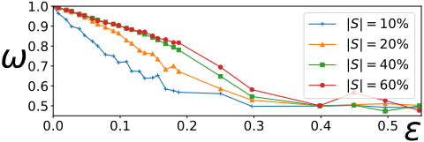
Starting from a linear function g : B8 → B defined as g(x) = x1 + · · · + x8, we introduce some noise by negating its output g(x) with probability ε. We obtain functions fε that are ε-close to the set of linear functions. In figure 1, we report the values of ω(S, fε) using the Standard modeling for different sizes of S (as a percentage of |Bm|). Results are averaged over 50 experiments. Other experiments have been carried out with other linear functions (i.e. with less essential variables or different arity), leading to very similar results. Note that ε only needs to be taken in [0, 12 ], because when g is ε-close to L, ¬g is (1 - ε)-close to L and they have the same ω, so the curves are symmetrical w.r.t. the axis ε = 1 2 .
When ε = 0 we get ω = 1, as expected from Proposition 3. We observe an almost linear decrease in ω as ε grows to 0.3 - 0.4 then leading to a plateau where ω = 12 , indicating that the analogical labels xf are more or less random. Moreover, ω appears to decrease faster for small samples S. This is due to the fact that the analogical labels xf are the result of a majority-vote procedure among the candidate solutions that one can build from S, and the number of candidates becomes smaller as |S| decreases, thus altering the quality of the prediction. The determination of a functional dependence between ω, ε and |S| is currently being investigated.
Now, let us note the following point: even if a function f is far from being AP, the quality ω of the extension ES(f) may still be very high. To illustrate this, let us define the value β which is an indicator of how far is f from being completely AP. For each x ∈ E∗S (f), we define βx as the proportion of candidates y that led to the correct label, i.e. the proportion of y such that y = f(x). β is defined as the average of all the βx. Obviously, a function f is AP iff β = 1 for all S, i.e. if βx = 1 for all x ∈ E∗S (f) and for all S.
Table 3 reports the values of ω and β for the Standard and the Klein modelings of analogy (respectively ωS , ωK, βS and βK) over three datasets from the UCI repository, namely the three Monk's problems 3 [Lichman, 2013]. Results are averaged over 100 experiments, where the sample set S is each time randomly sampled with a size that is 30% that of the universe of possible instances.
| ωS | ωK | βS | βK | |
|---|---|---|---|---|
| Monk 1 | .96 | .96 | .73 | .62 |
| Monk 2 | .96 | .84 | .69 | .60 |
| Monk 3 | .98 | .95 | .87 | .77 |
We observe that for each dataset, βS is significantly lower than 1. This suggests that the Boolean functions underlying these datasets are highly not AP, because on average, there is a high proportion (around 20%) of candidates y that predicted the wrong label. However, ωS is no lower than 96%, implying extensions of very high quality. This is where the majority-vote comes into play: in some cases, it may be able to compensate for the predictors y that were wrong. This is what happens here in 96%, 96% and 98% of the cases respectively. Here again, obtaining theoretical guarantees about the majority vote procedure is currently investigated.
We note also that the Klein modeling achieves equal or lower quality than the standard one, which suggests that the Standard modeling, which has the same class of AP functions, is more useful in practice. Note that such a difference between ωS and ωK has been consistently observed over many other experiments, which we do not mention here due to lack of space. This may be explained by the fact that, as mentioned earlier, the Klein modeling obeys the following property, unnatural for an analogy: AK(a, b, c, d) ⇐⇒ AK(b, a, c, d).
6 Conclusion and FutureWorks
In this paper, we have shown the interest of using analogical proportions for extending a Boolean sample set for classification purposes. We introduced the notion of AP functions, which are the functions underlying the labels of a dataset that ensure completely error-free extensions. After identifying the AP functions as the class of affine Boolean functions (that are all XOR-based functions), we discussed how these theoretical results could be of use in real-world problems.
We have investigated two ways of deviating from being AP for a function f. Firstly, by studying ε-close affine functions, and by observing changes in the quality of the extension. Secondly, by studying benchmark datasets that are clearly not AP, but that still achieve a high extension quality. These sets of experiments call for two topics of future research that arise from these observations. In both cases, it is a matter of exhibiting theoretical guarantees on the quality of the extension w.r.t. these two approximation hypotheses. Moreover, an expected generalization of the results reported here should apply to nominal attributes as well.
3 These datasets being nominally-valued, each feature with k nominal values is encoded using k binary features.
@inproceedings{ijcai2017p218,
  title     = {Analogy-preserving functions: A way to extend Boolean samples},
  author    = {Couceiro, Miguel and Hug, Nicolas and Prade, Henri and Richard, Gilles},
  booktitle = {Proceedings of the Twenty-Sixth International Joint Conference on
               Artificial Intelligence, {IJCAI-17}},
  publisher = {International Joint Conferences on Artificial Intelligence Organization},
  editor    = {Carles Sierra},
  pages     = {1575--1581},
  year      = {2017},
  month     = {8},
  note      = {Main track},
  doi       = {10.24963/ijcai.2017/218},
  url       = {https://doi.org/10.24963/ijcai.2017/218},
}
TY - CPAPER TI - Analogy-preserving functions: A way to extend Boolean samples AU - Couceiro, Miguel AU - Hug, Nicolas AU - Prade, Henri AU - Richard, Gilles T2 - Proceedings of the Twenty-Sixth International Joint Conference on Artificial Intelligence, IJCAI-17 PB - International Joint Conferences on Artificial Intelligence Organization PY - 2017 SP - 1575 EP - 1581 DO - 10.24963/ijcai.2017/218 UR - https://doi.org/10.24963/ijcai.2017/218 ER -Copied
Machine-readable versions of this paper, for tools and AI agents:





