
Optimal Feature Selection for Decision Robustness in Bayesian Networks
Proceedings of the Twenty-Sixth International Joint Conference on Artificial Intelligence. Main track. Pages 1554-1560.
https://doi.org/10.24963/ijcai.2017/215
Keywords
- Knowledge Representation, Reasoning, and Logic: Tractable languages and knowledge compilation
- Uncertainty in AI: Bayesian Networks
- Uncertainty in AI: Decision/Utility Theory
- Machine Learning: Feature Selection/Construction
Abstract
In many applications, one can define a large set of features to support the classification task at hand. At test time, however, these become prohibitively expensive to evaluate, and only a small subset of features is used, often selected for their information-theoretic value. For threshold-based, Naive Bayes classifiers, recent work has suggested selecting features that maximize the expected robustness of the classifier, that is, the expected probability it maintains its decision after seeing more features. We propose the first algorithm to compute this expected same-decision probability for general Bayesian network classifiers, based on compiling the network into a tractable circuit representation. Moreover, we develop a search algorithm for optimal feature selection that utilizes efficient incremental circuit modifications. Experiments on Naive Bayes, as well as more general networks, show the efficacy and distinct behavior of this decision-making approach.
- [Bache and Lichman, 2013] K. Bache and M. Lichman. UCI ma- chine learning repository, 2013.
- [Bellala et al., 2013] Gowtham Bellala, Jason Stanley, Suresh K. Bhavnani, and Clayton Scott. A rank-based approach to active diagnosis. IEEE Trans. Pattern Anal. Mach. Intell., 35(9):2078- 2090, 2013.
- [Bilgic and Getoor, 2011] Mustafa Bilgic and Lise Getoor. Value of information lattice: Exploiting probabilistic independence for effective feature subset acquisition. Journal of Artificial Intelli- gence Research (JAIR), 41:69-95, 2011.
- [Bova, 2016] Simone Bova. SDDs are exponentially more succinct than OBDDs. In Proceedings of the Thirtieth AAAI Conference on Artificial Intelligence, pages 929-935. AAAI Press, 2016.
- [Chavira and Darwiche, 2005] M. Chavira and A. Darwiche. Com- piling bayesian networks with local structure. In Proceedings of IJCAI, volume 5, pages 1306-1312, 2005. IJCAI
- [Chavira and Darwiche, 2008] M. Chavira and A. Darwiche. On probabilistic inference by weighted model counting. AIJ, 172(6- 7):772-799, 2008.
- [Chen et al., 2013] Suming Chen, Arthur Choi, and Adnan Dar- wiche. An exact algorithm for computing the Same-Decision Probability. In Proceedings of the 23rd International Joint Con- ference on Artificial Intelligence, pages 2525-2531, 2013. IJCAI
- [Chen et al., 2014] Suming Chen, Arthur Choi, and Adnan Dar- wiche. Algorithms and applications for the Same-Decision Probability. Journal of Artificial Intelligence Research (JAIR), 49:601-633, 2014.
- [Chen et al., 2015a] Suming Chen, Arthur Choi, and Adnan Dar- wiche. Computer adaptive testing using the same-decision proba- bility. In Proceedings of the Twelfth UAI Conference on Bayesian Modeling Applications Workshop, pages 34-43, 2015.
- [Chen et al., 2015b] Suming Chen, Arthur Choi, and Adnan Dar- wiche. Value of information based on Decision Robustness. In Proceedings of the 29th Conference on Artificial Intelligence (AAAI), 2015.
- [Choi et al., 2012] Arthur Choi, Yexiang Xue, and Adnan Dar- wiche. Same-Decision Probability: A confidence measure for threshold-based decisions. International Journal of Approximate Reasoning (IJAR), 2:1415-1428, 2012.
- [Choi et al., 2013] A. Choi, D. Kisa, and A. Darwiche. Compil- ing probabilistic graphical models using sentential decision dia- grams. In ECSQARU, pages 121-132, 2013.
- [Darwiche and Marquis, 2002] A. Darwiche and P. Marquis. A knowledge compilation map. JAIR, 17:229-264, 2002.
- [Darwiche et al., 2008] Adnan Darwiche, Rina Dechter, Arthur Choi, Vibhav Gogate, and Lars Otten. Results from the proba- blistic inference evaluation of UAI-08. http://graphmod. ics.uci.edu/uai08/Evaluation/Report, 2008. Link
- [Darwiche, 2009] Adnan Darwiche. Modeling and Reasoning with Bayesian Networks. Cambridge University Press, 2009.
- [Darwiche, 2011] A. Darwiche. SDD: A new canonical representa- tion of propositional knowledge bases. In Proceedings of IJCAI, pages 819-826, 2011. IJCAI
- [Dechter and Mateescu, 2007] Rina Dechter and Robert Mateescu. And/or search spaces for graphical models. Artificial intelligence, 171(2-3):73-106, 2007.
- [Fierens et al., 2015] Daan Fierens, Guy Van den Broeck, Joris Renkens, Dimitar Shterionov, Bernd Gutmann, Ingo Thon, Gerda Janssens, and Luc De Raedt. Inference and learning in probabilis- tic logic programs using weighted Boolean formulas. Theory and Practice of Logic Programming, 15:358-401, 5 2015.
- [Gao and Koller, 2011] T. Gao and D. Koller. Active classification based on value of classifier. In Advances in Neural Information Processing Systems (NIPS 2011), 2011.
- [Gimenez et al., 2014] Francisco J Gimenez, Yirong Wu, Eliza- beth S Burnside, and Daniel L Rubin. A novel method to assess incompleteness of mammography reports. In AMIA Annual Sym- posium Proceedings, volume 2014, page 1758. American Medi- cal Informatics Association, 2014.
- [Heckerman et al., 1993] David Heckerman, Eric Horvitz, and Blackford Middleton. An approximate nonmyopic computation for value of information. IEEE Transactions on Pattern Analysis and Machine Intelligence, 15(3):292-298, 1993.
- [Huang et al., 2006] Jinbo Huang, Mark Chavira, Adnan Darwiche, et al. Solving map exactly by searching on compiled arithmetic circuits. In AAAI, volume 6, pages 3-7, 2006.
- [Korf, 2009] Richard E Korf. Multi-way number partitioning. In IJCAI, pages 538-543. Citeseer, 2009. IJCAI
- [Krause and Guestrin, 2009] Andreas Krause and Carlos Guestrin. Optimal value of information in graphical models. Journal of Artificial Intelligence Research (JAIR), 35:557-591, 2009.
- [Malings and Pozzi, 2016] Carl Malings and Matteo Pozzi. Condi- tional entropy and value of information metrics for optimal sens- ing in infrastructure systems. Structural Safety, 60:77-90, 2016.
- [Millán and Pérez-De-La-Cruz, 2002] Eva Millán and José Luis Pérez-De-La-Cruz. A Bayesian diagnostic algorithm for student modeling and its evaluation. User Modeling and User-Adapted Interaction, 12(2-3):281-330, 2002.
- [Munie and Shoham, 2008] Michael Munie and Yoav Shoham. Op- timal testing of structured knowledge. In Proceedings of the 23rd National Conference on Artificial intelligence, pages 1069-1074, 2008.
- [Oztok et al., 2016] Umut Oztok, Arthur Choi, and Adnan Dar- wiche. Solving PP PP -complete problems using knowledge com- pilation. In Proceedings of the 15th International Conference on Principles of Knowledge Representation and Reasoning (KR), pages 94-103, 2016.
- [Sang et al., 2005] Tian Sang, Paul Beame, and Henry A Kautz. Performing bayesian inference by weighted model counting. In AAAI, volume 5, pages 475-481, 2005.
- [Selman and Kautz, 1996] Bart Selman and Henry Kautz. Knowl- edge compilation and theory approximation. Journal of the ACM (JACM), 43(2):193-224, 1996.
- [Van den Broeck and Darwiche, 2015] G. Van den Broeck and A. Darwiche. On the role of canonicity in knowledge compi- lation. In Proceedings of the 29th Conference on Artificial Intel- ligence (AAAI), 2015.
- [Yu et al., 2009] Shipeng Yu, Balaji Krishnapuram, Romer Ros- ales, and R Bharat Rao. Active sensing. In International Con- ference on Artificial Intelligence and Statistics, pages 639-646, 2009.
- [Zhang and Ji, 2010] Yongmian Zhang and Qiang Ji. Efficient sen- sor selection for active information fusion. IEEE Transactions on Systems, Man, and Cybernetics, Part B, 40(3):719-728, June 2010.
References were extracted automatically from the PDF and may contain errors.
Full text extracted automatically from the PDF; figures, tables and equations may differ. The PDF is the version of record.
1 Introduction
Classification and Bayesian decision making are complicated by the fact that features - the input to our decision making process - are expensive to evaluate in many application domains. In medical diagnosis, cost prohibits the doctor from running all possible tests, necessitating selective and active sensing [Yu et al., 2009]. Similar issues arise in sensor networks [Krause and Guestrin, 2009], adaptive testing [Mill´an and P´erez-De-La-Cruz, 2002; Munie and Shoham, 2008], network diagnosis [Bellala et al., 2013], and seismic risk monitoring [Malings and Pozzi, 2016].
Traditionally, such problems have been tackled by selecting features that optimize the decision-theoretic value of information [Heckerman et al., 1993; Bilgic and Getoor, 2011]. These approaches seek to maximize the expected reward of observing the features. In one common instance, this means observing features that maximize the information gain, or equivalently, minimize the conditional entropy of the variable of interest (e.g., the medical diagnosis) [Zhang and Ji, 2010; Gao and Koller, 2011]. We refer to Krause and Guestrin [2009] for a more detailed discussion.
Another criterion called same-decision probability (SDP) came to the front more recently [Choi et al., 2012; Chen et al., 2014]. Given a current set of observed features, and the corresponding threshold-based decision, the SDP measures the robustness of this decision against further observations. It is the probability that our classification will be unchanged after all remaining features are revealed. SDP was successfully used to evaluate mammography-based diagnosis [Gimenez et al., 2014] and adaptive testing [Chen et al., 2015a].
Chen et al. [2015b] propose to use decision robustness for feature selection. In this context, we need to evaluate the expected robustness of a future decision based on the selected subset of features. It is compared to the hypothetical decision based on all features. The probability that these two classifiers agree is the expected SDP.
As our first contribution, we present the first algorithm to compute the expected SDP query on general Bayesian networks, which is PP PP -complete [Choi et al., 2012]. 1 Previous expected SDP algorithms were restricted to Naive Bayes networks, where computing the SDP is (only) NP-hard [Chen et al., 2013], and is amenable to heuristic search. Our expected SDP algorithm is instead based on the knowledge compilation approach of Oztok et al. [2016] for solving PP PP -complete problems using sentential decision diagrams (SDDs) [Darwiche, 2011].
Our second contribution is an optimal feature selection algorithm. It searches for the subset of features that fits in our budget and is maximally robust according to expected SDP. The algorithm incrementally modifies an SDD representation of the Bayesian network during search, in order to efficiently re-evaluate the expected SDP of a large number of feature sets. It is the first optimal feature selection algorithm for general Bayesian network classifiers that optimizes robustness.
As a third contribution, we illustrate how decision robustness leads to different feature selection behavior on general Bayesian networks, compared to value of information. Moreover, the feature selection behavior depends strongly on the threshold used - a distinct property of the expected SDP criterion. We demonstrate our feature selection algorithm on both naive Bayes and general Bayesian network classifiers.
1 Note that NP ⊆ PP ⊆ NP PP ⊆ PP PP ⊆ PSPACE ⊆ EXPTIME. MPE queries (NP), marginal probabilities (PP), and marginal MAP (NP PP ) are all easier than (expected) SDP queries [Darwiche, 2009].
| Pr(D=+) | D | Pr(R1 =+|D) |
|---|---|---|
| 0.2 | + - | 0.7 0.2 |
| D R1 R2 | D + - | Pr(R2 =+|D) 0.6 0.1 |
| R1 R2 | Pr(AC=+|R1R2 ) | |
| AC | + + + - - + | 0.9 0.2 0.3 |
| - - | 0 |
2 Same-Decision Feature Selection
We write uppercase letters for random variables and lowercase letters for their instantiation. Sets of variables are written in bold uppercase, and their joint instantiation in bold lowercase. Concatenations of sets denote their union (e.g. XY).
2.1 Motivation and Intuition
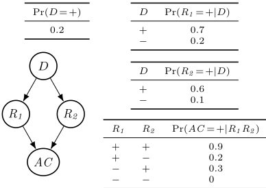
Imagine a scenario where a program chair (PC) wants to determine the true quality D of a submitted paper. Two reviewers, R1 and R2 , independently evaluate the paper, and their assessments are summarized by area chair AC. Figure 1 depicts this scenario as a Bayesian network. The PC wants to ascertain that accepted papers are high quality with at least 60% probability. This means that papers with two positive reviews get accepted regardless of the AC's evaluation, as
and all other papers get rejected. We refer to this ideal classifier as C ⋆ . In practice, however, the PC only has time to observe a single evaluation. The question then is: which feature should the decision be based on; R1 , R2 , or AC?
This scenario gives rise to three possible classifiers, CR1 , CR2 , and CAC , depending on which feature is selected. For our threshold of 60%, these make the following decisions.
It is customary to evaluate these classifiers with informationtheoretic measures, such as information gain, or equivalently, the conditional entropy H(D|F ) of D given feature F :
where h(p) is the entropy of a Bernoulli with probability p. This tells us that CR2 is the best classifier, yielding most certainty about D, and the area chair's review CAC is the worst, providing the least amount of information (i.e., high entropy).
Nevertheless, our PC may not want to maximize information content, and may simply strive to make the same decisions as the ones made by the ideal classifier C ⋆ . The most informative classifier CR2 agrees with the optimal classifier on 90% of the papers, in all cases except when R1 =- and R2 =+. Classifier CR1 also makes the same decision in 90% of the cases. Our least informative classifier CAC , however, outperforms both. When it rejects a paper because AC =-, the ideal classifier C ⋆ agrees 99% of the time, namely in those cases where the AC did not overrule the reviewers. When CAC accepts a paper because AC =+, the ideal classifier C ⋆ agrees 56% of the time, in those cases where the reviewers both voted accept. These quantities are called same-decision probabilities. Overall, we expect CAC to make the same decisions as C ⋆ on 92% of the papers, which is its expected same-decision probability.
In conclusion, to optimize the decision, the PC should follow the AC evaluation, not an individual reviewer, even though their evaluations contain more information.
2.2 Problem Statement
Next, we formalize the robustness of a current decision against future observations as the same-decision probability.
Definition 1. Let d and e be instantiations of the decision variable D and evidence variables E. Let T be a threshold. Let X be a set of variables distinct from D and E. The samedecision probability (SDP) in distribution Pr is
Here, the equality =T holds if both sides evaluate to a probability on the same side of threshold T , and [α] is 1 when α is true and 0 otherwise.
Expected SDP measures the redundancy of a feature set X if we were to first observe another feature set Y.
Definition 2. Let d and e be instantiations of the decision variable D and evidence variables E. Let T be a threshold. Let X and Y be disjoint sets of variables. The expected samedecision probability (E-SDP) in distribution Pr is
We will drop subscripts d and T when clear from context.
In same-decision feature selection, we are given a set of candidate features F, a positive cost function c(.), and budget B. The goal is to find features Y ⊆ F maximizing SDPd,T ((F \Y) | Y, e), subject to a cost constraint ∑Y ∈Y c(Y ) ≤ B. That is, we select those features that fit in our budget and maximize the decision robustness, measured by expected SDP against the remaining features that were not selected.
3 A Tractable Circuit Representation
This section describes the logical foundation of our algorithms. Modern approaches to discrete probabilistic inference often reduce the problem to a logical one, encoding the distribution in weighted propositional logic [Chavira and Darwiche, 2005; 2008; Sang et al., 2005; Dechter and Mateescu, 2007; Fierens et al., 2015]. This technique naturally exploits structure in the distribution such as determinism and context-specific independence, and attains state-of-theart performance [Darwiche et al., 2008; Choi et al., 2013]. In particular, we follow the knowledge compilation approach, where one compiles the logical description of the inference problem into a tractable (circuit) representation [Selman and Kautz, 1996; Darwiche and Marquis, 2002]. Knowledge compilation is particularly useful to solve some of the harder reasoning problems in AI, referred to as problems "beyond NP". 2 These include problems that are PP-hard, NP PP -hard, or even PP PP -hard, while still being of significant practical interest [Huang et al., 2006; Oztok et al., 2016]. SDP and E-SDP queries belong to this family.
Notation We employ the same notation for propositional logic variables and random variables, as well as for their instantiations. A literal is a variable or its negation. Logical sentences are constructed in the usual way. Abusing notation, an instantiation can denote its corresponding set or conjunction of literals. A model x of a sentence α over variables X is a complete instantiation of X that satisfies α, denoted x |= α. Conditioning α|x substitutes all X in α by their values in x.
3.1 Encoding inWeighted Propositional Logic
Several encodings have been proposed to reduce Bayesian networks into (i) a propositional sentence α, and (ii) a function w(.) that maps literals to weights. Variables Z in α come from two disjoint sets: indicators I and parameters P, corresponding to values of network variables and network parameters, respectively. Literals ℓ constructed from I are assumed to have w(ℓ) = 1. We refer to Chavira and Darwiche [2008] for the technical details and alternatives. Here, we instead show a simple encoding of the CPT for Pr(R1 |D) in Figure 1, which reduces to the sentence αR1 |D consisting of
and its associated weight function sets w(P1) = 0.7, w(P2) = 0.3, w(P3) = 0.2, w(P4) = 0.8, and all other weights to 1. The full encoding α is obtained by conjoining the sentences for each CPT.
The logical task called weighted model counting (WMC) sums the weight of all models of α that we are interested in:
We omit w when clear from context and write φα for φα(⊤). Given a weighted propositional logic encoding (α, w) of Pr, inference of conditional probabilities reduces to WMC. Indeed, Pr(x|e) = φwα (x|e), where x and e are variable instantiations, encoded using indicators from I.
2 http://beyondnp.org/
- (a) Sentential decision diagram (SDD)
(b) Variable tree (vtree)
Figure 2: Tractable SDD circuit representation for Sentence 1
3.2 Sentential Decision Diagrams
Sentential decision diagrams (SDDs) [Darwiche, 2011] are a knowledge compilation target language that allows for efficient WMC inference and incremental modifications (conjunction, disjunction, and conditioning of circuits) [Van den Broeck and Darwiche, 2015], which our algorithms will make use of. At the same time, SDDs are the most compact representation known to have these properties, exponentially smaller than ordered binary decision diagrams (OBDDs) [Bova, 2016].
Partitions SDDs are based on a new type of decomposition, called (X,Y)-partitions. Consider a sentence α and suppose that we split its variables into two disjoint sets, X and Y. It is always possible to decompose the sentence α as
Sentences pi are called primes, and are mutually exclusive, exhaustive, and consistent. Sentences si are called subs.
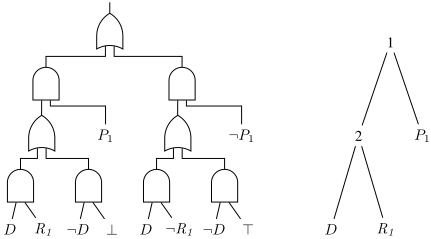
For example, consider Sentence 1 in our encoding of Pr(R1 |D). By splitting the variables into X = {D,R1} and Y = {P1}, we obtain the (X, Y)-partition
The primes are indeed mutually exclusive, exhaustive and non-false. This partition is represented in terms of logical gates by the top two layers of the SDD circuit in Figure 2a. In the graphical depiction of SDDs, primes and subs are either a constant, a literal or an input wire from another gate.
Vtrees SDDs represent a sequence of recursive (X,Y)- partitions. To build an SDD, we need to determine which X and Y are used in every partition in the SDD. This process is governed by a variable tree (vtree): a full, binary tree, whose leaves are labeled with variables; see Figure 2b. The root v of the vtree partitions variables into those appearing in the left subtree (X) and those appearing in the right subtree (Y). This implies an (X,Y)-partition of sentence α, leading to the top two layers in Figure 2a. We say that the SDD's root node is normalized for vtree node v. The primes and subs of this partition are turned into SDDs, recursively, normalized
Algorithm 1 SDPd,T (X | Y, e)
Input:
d : hypothesis; T : threshold; e : evidence
X,Y : disjoint sets of features
S : Y-constrained and XY-constrained SDD
Output: computes SDPd,T (X | Y, e)
1: for each SDD node α in S (children before parents) do 2: if α is a terminal then 3: vr1(α) ← φα if α ∼ e; else 0 4: vr2(α) ← φα if α ∼ de; else 0 5: else 6: vr 1(α) ← ∑(pi ,si)∈α vr 1(pi) × vr 1(si) 7: vr 2(α) ← ∑(pi ,si)∈α vr 2(pi) × vr 2(si) 8: for each SDD node α in S (children before parents) do 9: if α is a terminal then 10: vr 3(α) ← φα 11: else if α is XY-constrained then 12: β ← Y-constrained ancestor of α 13: vr3(α) ← vr1(α) if vr2(α) vr1(α) =T vr 2(β) vr1(β) ; else 0 14: else 15: vr 3(α) ← ∑(pi ,si)∈α vr 3(pi) × vr 3(si) 16: φ(e) ← vr1(S); Q← vr3(S) 17: return Q/φ(e)for vtree nodes from the left and right subtrees. The process continues until we reach variables or constants. The vtree used to construct an SDD can have a dramatic impact on its size, sometimes leading to an exponential difference.
4 Computing the Expected SDP with SDDs
We now introduce our approach to compute E-SDP by compilation into SDDs. As described in Section 3, we can encode a Bayesian network into weighted propositional logic (α, w) and further compile it into an SDD. Then, computing the ESDP over a set of features translates to computing the E-SDP over a set of variables of its circuit encoding.
Definition 3. Let d and e be instantiations of the decision variable D and evidence variables E. Let T be a threshold. Let X and Y be disjoint sets of variables. The expected samedecision probability on a WMC encoding (α, w) of Pr is
Our approach to compute the E-SDP using SDDs is shown in Algorithm 1. It requires a special type of SDDs that are normalized for constrained vtrees [Oztok et al., 2016].
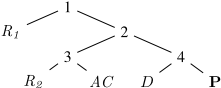
Definition 4. A vtree node v is X-constrained, denoted vX, iff it appears on the right-most path of the vtree and X is exactly the set of variables outside v. A vtree is X-constrained iff it has an X-constrained node. An SDD is X-constrained iff it is normalized for an X-constrained vtree. An SDD node is X-constrained iff it is normalized for vX.
In order to compute SDPd,T (X|Y, e), we require an SDD that is Y-constrained and XY-constrained. That is, we need an SDD that is normalized for a vtree with a Y-constrained node and an XY-constrained node. Figure 3 depicts an example of such a vtree, which would allow us to compute SDP(R2 ,AC | R1 ). Note that the Y-constrained node is always an ancestor of XY-constrained node.
The algorithm performs two bottom-up passes over the SDD and keeps three value registers for each SDD node. In the first pass (Lines 1-7), it computes the weighted model counts of each SDD node with respect to instantiations e and de, and saves the results in value registers, analogous to the SDP algorithm of Oztok et al. [2016].
Lemma 1. Let α be an SDD node normalized for vtree v. Then, vr1(α) = φα(ev) and vr2(α) = φα(dvev), where ev and dv denote the subset of instantiation e and d, respectively, that pertains to the variables of vtree v.
During the second bottom-up pass (Lines 8-15), the algorithm simply computes a weighted model count for any SDD node α that is neither an XY-constrained node nor its ancestor. Next, if α is normalized for vXY, then α must equal S|xy for some instantiations x and y. Also, its Y-constrained ancestor β must equal S|y. Then Line 13 computes the function [φα(d | e) =T φβ(d | e)] φα(e). We can use induction on the distance of v to vXY to show that the following holds.
Lemma 2. Let α be an SDD node normalized for vtree v, where v is vXY or one of its ancestors, but v is not an ancestor of vY. Let β be the Y-constrained ancestor of α (that is, β is normalized for vY). Then,
It follows from above lemma that at the Y-constrained SDD node α, our algorithm computes the following quantity:
We can again use induction on the distance of v to vY to show the following.
Lemma 3. Let α be an SDD node normalized for vtree v, where v is vY or one of its ancestors. Then,
The complete proofs of above lemmas are found in the appendix. Line 16 now computes the quantity
Algorithm 2 FS-SDD(Q, d, b)
Input:
d : hypothesis; T : threshold;
e : evidence;
B : budget;
F : {F1, . . . , Fn}, set of features
c : cost function; S : F-constrained SDD
Data:
Q← {} : features selected
k ← 0 : depth b ←B : budget left
Y : best subset p : best E-SDP
Output: Subset Y ⊆ F with best E-SDP within budget B
1: if b < 0 then return 2: else if k > n then return 3: else if c(Fk) ≤ b then 4: Z←Q∪ {Fk} 5: move variable in S to make it Z-constrained 6: if SDP((F \ Z) | Z, e) > p then 7: Y ← Z 8: p ← SDP((F \ Z) | Z, e) 9: FS-SDD(Z, k +1, b - c(Fk)) 10: FS-SDD(Q, k +1, b)Dividing Q by vr 1(S) = φS(e) yields the expected SDP.
Note that the algorithm performs a constant amount of work at each SDD node. Thus, we have the following.
Proposition 2. Alg. 1 runs in time linear in the size of SDD S.
5 Feature Selection using SDDs
A naive approach to feature selection computes E-SDP for each possible subset of features that respects the budget and chooses the best one. However, this requires exponentially many compilations of SDDs since our E-SDP algorithm expects a different Y-constrained SDD for each subset Y.
We can improve upon this approach by introducing an operation to move a variable within a vtree and adjusting the SDD accordingly. Suppose we want to move a variable X of an SDD α, normalized for vtree v. If we condition α on X being true, the resulting SDD β = α|X no longer contains the variable X. Similarly, we can obtain an SDD for γ = α|¬X. Since X is not used for β and γ, we can move it to a new location to obtain a new vtree v′ , and β and γ will still be normalized for vtree v′ . Finally, we join them to get a new SDD α′ = (X ∧ β) ∨ (¬X ∧ γ), using an efficient APPLY function [Darwiche, 2011; Van den Broeck and Darwiche, 2015], which is normalized for vtree v′ and still represents the same Boolean formula as α. Thus, once we compile an SDD, we can move variables around to make a Y-constrained node for each subset Y, instead of recompiling the SDD.
Our proposed algorithm FS-SDD, shown in Algorithm 2, generates candidate subsets by depth-first searching an inclusion-exclusion tree, as described in Korf [2009] and Chen et al. [2015b]. At each depth of the tree, we either include or exclude the variable pertaining to that depth in the subset. We backtrack if the cost so far exceeds the budget. Each time we include a variable in the subset, the expected SDP over that subset is computed using Algorithm 1, updating the optimal subset and its E-SDP as necessary.
Note that we are interested in computing the exact value of E-SDP only if it exceeds the highest E-SDP computed for some previous subset. Thus, we can early terminate the computation and continue our search to the next candidate, if an upper bound for current E-SDP falls below the highest value so far. We can do this by adding the following after line 13 of Algorithm 1: if vr3(α) = 0 then ub ← ub - vr1(α) vr 1(S) ; if ub < best esdp then return. At the start of each E-SDP computation, ub is initialized to 1, and best esdp is set to the highest E-SDP value until that point in search.
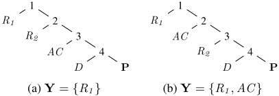
Analysis We illustrate that moving a variable each search iteration of FS-SDD is efficient, if the input SDD S is normalized for a vtree that is right-linear outside of its Fconstrained node. 3 For example, for F = {R1 ,R2 ,AC}, Figure 4a satisfies this requirement, but Figure 3 does not. Each time we compute E-SDP over Z = Q ∪ {Fk}, we already have a Q-constrained node from the last recursive step, and variable Fk should appear inside the Q-constrained vtree but outside the F-constrained vtree. We can simply move Fk, using the operation defined previously, right after the nth variable in the vtree where n is the size of Q. Figure 4 gives an example of such operation where Q = {R1} and Fk = AC. In other words, the F variables appear in the same order in the vtree as in the path to the current search point in the inclusion-exclusion tree. This also maintains the right-linear structure outside the F-constrained node, so we only need to move one variable in each search step.
6 Experimental Evaluation
We now empirically evaluate our SDD-based approach for decision-robust feature selection.
Naive Bayes We evaluated our system on Naive Bayes networks from the UCI repository [Bache and Lichman, 2013], BFC (http://www.berkeleyfreeclinic. org/), and CRESST (http://www.cse.ucla.edu/). We performed experiments using three variations of our SDD-based algorithm. We compare to MAXDR which, to our knowledge, is the only exact algorithm for feature selection based on E-SDP [Chen et al., 2015b]. Since both algorithms find exact solutions, we compare their running times.
3 A vtree is right-linear if each left child is a leaf.
| Network | |F| | MaxDR | FS-SDD1 | FS-SDD2 | FS-SDD3 |
|---|---|---|---|---|---|
| bupa | 6 | 0.021 | 0.184 | 0.035 | 0.044 |
| pima | 8 | 0.033 | 0.372 | 0.058 | 0.056 |
| ident | 9 | 0.105 | 1.548 | 0.127 | 0.128 |
| anatomy | 12 | 2.393 | 35.720 | 2.951 | 2.252 |
| heart | 13 | 18.649 | 122.822 | 9.907 | 6.321 |
| voting | 16 | 682.396 | timeout | 1110.96 | 810.042 |
| Network | # nodes | naive | FS-SDD |
|---|---|---|---|
| alarm | 37 | 143.920 | 19.061 |
| win95pts | 76 | 23.581 | 14.732 |
| tcc4e | 98 | 48.508 | 2.384 |
| emdec6g | 168 | 28.072 | 3.688 |
| diagnose | 203 | 105.660 | 6.667 |
For each network, we find the optimal subset for E-SDP with the budget set to 1/3 the number of features. In all experiments, the cost of each feature is 1, timeout is 1 hour, and a 2.6GHz Intel Xeon E5-2670 CPU with 4GB RAM was used. FS-SDD1 refers to the naive approach that compiles a constrained SDD for every candidate subset. FS-SDD2 directly compiles the network into an F-constrained SDD which is then passed into our FS-SDD algorithm. Lastly, FS-SDD3 first compiles an unconstrained SDD and, after compilation, moves variables to make it F-constrained. Table 5 shows that the naive approach performs worst. This highlights that repeated SDD compilation is very expensive. Moreover, FSSDD3 outperforms FS-SDD2 as network size increases, illustrating that directly compiling a constrained SDD can be challenging for large networks and that moving variables is more effective. Moreover, even though MAXDR outperforms SDD-based approaches in most of the benchmarks, the running times of MAXDR and FS-SDD3 are comparable. Thus, utilizing efficient SDD operations enables our generalpurpose algorithm to perform as well as MAXDR which is designed specifically for Naive Bayes networks.
General Bayesian Networks We now evaluate our algorithm on general Bayesian networks provided by HRL Laboratories and benchmarks from the UAI 2008 evaluation. For each network, a decision variable was chosen at random from root nodes, and 10 variables were randomly selected to be our set of features F. We used FS-SDD to select an optimal subset of size at most 3. As this is the first algorithm for feature selection using E-SDP in general Bayesian networks, we compare our algorithm to a naive, brute-force approach which enumerates all possible instantiations of features to compute the E-SDP. Table 6 shows that our algorithm runs significantly faster than the naive approach, and that it performs as well on larger general Bayesian networks as it does on Naive Bayes networks. To calculate the marginals for the brute-force approach, we used jointree inference as implemented in SAMIAM. 4 Note that the runtime of the jointree algorithm is exponential in the treewidth of the network, whereas the SDD approach can sometimes run efficiently on high-treewidth networks. [Choi et al., 2013] We also want to stress that the running time includes initial SDD compilation time, which in practice would be performed in an offline phase. Once we compile a constrained SDD, we can make observations and find the next optimal subset in an online fashion, thereby making decisions in a sequential manner.
4 SAMIAM is available at http://reasoning.cs.ucla. edu/samiam.
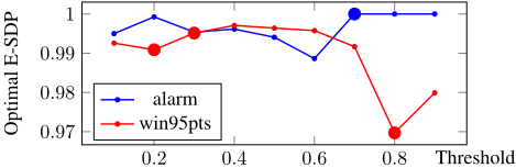
Threshold-Based Decisions Lastly, we demonstrate that decision robustness is not only a function of the probability distribution and features but also of the threshold, unlike other measures of value of information. For networks alarm and win95pts, we used FS-SDD to select features Y ⊆ F where F is the set of all leaf nodes in each network. No evidence was asserted, the decision variable was chosen randomly from root nodes, and the budget was set to 1/3 the size of F. Using the same decision variable, we repeatedly evaluated our algorithm with decision thresholds in {0.1, 0.2, . . . , 0.9}. Figure 7 shows different values of E-SDP for different thresholds. In fact, FS-SDD selects different features as the threshold changes. For example, a subset of three leaf nodes is chosen as an optimal subset for alarm for T ∈ [0.1, 0.6], whereas one leaf node can achieve expected SDP of 1.0 for T ∈ [0.7, 1.0]. Intuitively, the E-SDP measures redundancy of remaining features given a selected set of features, taking into account the decision procedure defined by the threshold. On the other hand, other measures such as information gain are unaware of the decision procedure and choose the same features regardless of changes in threshold.
7 Conclusion
We presented the first algorithm to compute the expected same-decision probability on general Bayesian network, as well as the first algorithm to use this measure of decision robustness for feature selection on general networks. This approach yields distinct results from other selection criteria. Our algorithms exploit the properties of sentential decision diagrams to evaluate and search feature sets efficiently.
Acknowledgments
This work is partially supported by NSF grants #IIS-1514253, #IIS-1657613, and #IIS-1633857, ONR grant #N00014-151-2339 and DARPA XAI grant #N66001-17-2-4032. The authors thank Arthur Choi for helpful discussions.
@inproceedings{ijcai2017p215,
  title     = {Optimal Feature Selection for Decision Robustness in Bayesian Networks},
  author    = {Choi, YooJung and Darwiche, Adnan and Van den Broeck, Guy},
  booktitle = {Proceedings of the Twenty-Sixth International Joint Conference on
               Artificial Intelligence, {IJCAI-17}},
  publisher = {International Joint Conferences on Artificial Intelligence Organization},
  editor    = {Carles Sierra},
  pages     = {1554--1560},
  year      = {2017},
  month     = {8},
  note      = {Main track},
  doi       = {10.24963/ijcai.2017/215},
  url       = {https://doi.org/10.24963/ijcai.2017/215},
}
TY - CPAPER TI - Optimal Feature Selection for Decision Robustness in Bayesian Networks AU - Choi, YooJung AU - Darwiche, Adnan AU - Van den Broeck, Guy T2 - Proceedings of the Twenty-Sixth International Joint Conference on Artificial Intelligence, IJCAI-17 PB - International Joint Conferences on Artificial Intelligence Organization PY - 2017 SP - 1554 EP - 1560 DO - 10.24963/ijcai.2017/215 UR - https://doi.org/10.24963/ijcai.2017/215 ER -Copied
Machine-readable versions of this paper, for tools and AI agents:





