
Compiling Bayesian Networks with Local Structure
Proceedings of the Nineteenth International Joint Conference on Artificial Intelligence. Pages 1306-1311.
© 2005 International Joint Conferences on Artificial Intelligence
Abstract
Recent work on compiling Bayesian networks has reduced the problem to that of factoring CNF encodings of these networks, providing an expressive framework for exploiting local structure. For networks that have local structure, large CPTs, yet no excessive determinism, the quality of the CNF encodings and the amount of local structure they capture can have a significant effect on both the offline compile time and online inference time. We examine the encoding of such Bayesian networks in this paper and report on new findings that allow us to significantly scale this compilation approach. In particular, we obtain order–of–magnitude improvements in compile time, compile some networks successfully for the first time, and obtain orders– of–magnitude improvements in online inference for some networks with local structure, as compared to baseline jointree inference, which does not exploit local structure.
- [Bacchus et al., 2003] Fahiem Bacchus, Shannon Dalmao, and Toniann Pitassi. Algorithms and complexity results for #SAT and Bayesian inference. In FOCS, pages 340- 351, 2003.
- [Boutilier et al., 1996] Craig Boutilier, Nir Friedman, Moisés Goldszmidt, and Daphne Koller. Context-specific independence in bayesian networks. In UAI'96, pages 115-123, 1996.
- [Chavira et al., 2004] M. Chavira, A. Darwiche, and M. Yaeger. Compiling relational bayesian networks for exact inference. In PGM-2004, pages 49-56, 2004.
- [Davis et al., 1962] Martin Davis, George Logemann, and Donald Loveland. A machine program for theorem prov- ing. Journal of the ACM, (5)7:394-397, 1962.
- [Darwiche, 2001a] Adnan Darwiche. Decomposable nega- tion normal form. Journal of the ACM, 48(4):608-647, 2001.
- [Darwiche, 2001b] Adnan Darwiche. Recursive condition- ing. Artificial Intelligence, 126(1-2):5-41, 2001.
- [Darwiche, 2002] Adnan Darwiche. A logical approach to factoring belief networks. In Proceedings of KR, pages 409-420, 2002.
- [Darwiche, 2003] Adnan Darwiche. A differential approach to inference in bayesian networks. JACM, 50(3):280-305, 2003.
- [Darwiche, 2004] Adnan Darwiche. New advances in com- piling CNF to decomposable negational normal form. In ECAI'2004.
- [Jensen et al., 1990] F. V. Jensen, S.L. Lauritzen, and K.G. Olesen. Bayesian updating in recursive graphical models by local computation. Computational Statistics Quarterly, 4:269-282, 1990.
- [Park and Darwiche, 2003] James Park and Adnan Dar- wiche. A differential semantics for jointree algorithms. NIPS 15, volume 1, pages 299-307. MIT Press, 2003.
- [Poole and Zhang, 2003] D. Poole and N.L. Zhang. Exploit- ing contextual independence in probabilistic inference. Journal of Artificial Intelligence, 18:263-313, 2003.
- [Shenoy and Shafer, 1986] Prakash P. Shenoy and Glenn Shafer. Propagating belief functions with local computa- tions. IEEE Expert, 1(3):43-52, 1986.
References were extracted automatically from the PDF and may contain errors.
Full text extracted automatically from the PDF; figures, tables and equations may differ. The PDF is the version of record.
1 Introduction
It was shown recently that compiling Bayesian networks corresponds to factoring multi-linear functions (MLFs) [Darwiche, 2003]. In particular, each Bayesian network can be characterized by an MLF of exponential size, whose evaluation and differentiation solves the exact inference problem. Moreover, the MLF can be factored into an arithmetic circuit (AC) whose size is not necessarily exponential, allowing one to use ACs as a compiled representation of Bayesian networks. Interestingly, [Park and Darwiche, 2003] has shown that building a jointree [Jensen et al., 1990; Shenoy and Shafer, 1986] for a Bayesian network corresponds in a precise sense to a process of factoring the MLF into an AC, which is embedded by the jointree structure.
These findings created new possibilities for performing exact inference, as they provided a new computational framework based on factoring MLFs. In fact, a specific MLF factoring method was proposed in [Darwiche, 2002], which can exploit the structure inherent in network parameters. According to this approach, one encodes the MLF using a propositional theory in Conjunctive Normal Form (CNF), factors the CNF, and then immediately extracts the AC from the CNF factorization. The benefit of this logical approach is twofold. First, it allows one to encode local structure in the form of determinism and context specific independence (CSI) [Boutilier et al., 1996]. For example, using this approach, it became practical to compile some Bayesian networks with binary variables and excessive determinism (induced by relational models) and having treewidths in excess of 200 by compiling the AC in minutes and evaluating them in seconds [Chavira et al., 2004]. The second advantage of this approach is its ability to accommodate different representations of conditional probability tables (CPTs) (decision trees, rules, noisy-or, etc.), without the need for algorithmic change. In this paper, we consider only tabular representations.
The critical computational step in the above approach is clearly that of factoring/compiling the CNF, which is done using an exhaustive and refined version of the DPLL algorithm [Davis et al., 1962; Darwiche, 2004]. The key observation underlying this paper is that the efficiency of the factoring step-both factoring time and size of factorization-can be significantly improved through careful CNF encodings which capture as much local structure as possible, and by passing additional information about these CNFs to the factoring algorithm. This becomes especially true when handling networks that have local structure, large CPTs, yet no excessive determinism. We do indeed propose a particular CNF encoding which appears quite effective on networks with such properties. We also identify a key semantic property of the resulting CNFs, which we exploit in the CNF factoring algorithm. By incorporating these findings, we show dramatic improvements in the both offline compile time and online inference. In the offline compilation phase, we get an order-ofmagnitude improvement in some cases and an ability to compile some networks for the first time. In the online phase, we observe orders-of-magnitude improvements on some well known benchmarks, such as Pathfinder, Munin1, and Water, over online inference by the baseline jointree algorithm.
2 FactoringMulti-linear Functions
Our investigation is based on three technical observations [Darwiche, 2003]: that every Bayesian network can be interpreted as an exponentially-sized MLF whose evaluation and differentiation solves the exact inference problem; that such an MLF can be factored into an AC whose size may not be ex-
| row | A | B | C | Pr(c | | a, b) |
|---|---|---|---|---|---|
| B 1 2 3 4 5 6 7 8 | a1 | b1 | c1 | θc1|a1b1 = | 0 |
| A | a1 | b1 | c2 | θc2|a1b1 = | 0.5 |
| a1 | b1 | c3 | θc3|a1b2 = | 0.5 | |
| a1 | b2 | c1 | θc1|a1b2 = | 0.2 | |
| C | a1 | b2 | c2 | θc2|a1b1 = | 0.3 |
| a1 | b2 | c3 | θc3|a1b1 = | 0.5 | |
| a2 | b1 | c1 | θc1|a2b2 = | 0 | |
| a2 | b1 | c2 | θc2|a2b2 = | 0 | |
| 9 | a2 | b1 | c3 | θc3|a2b1 = | 1 |
| 10 | a2 | b2 | c1 | θc1|a2b1 = | 0.2 |
| 11 | a2 | b2 | c2 | θc2|a2b2 = | 0.3 |
| 12 | a2 | b2 | c3 | θc3|a2b2 = | 0.5 |
1
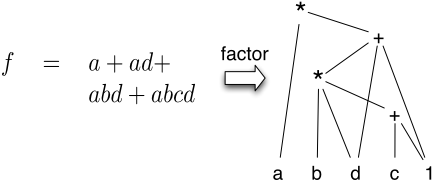
Figure 2: An MLF factored into an AC.
ponential; and that the MLF factoring process can be reduced to factoring a CNF encoding of the MLF.
The MLF for a network contains two types of variables. For each value x of each network variable X, there is an indicator variable λx. For each network parameter Pr(x|u), there is a parameter variable θx|u. The MLF contains a term for each instantiation of the network variables, and the term is the product of all indicators and parameters that are consistent with the instantiation. For the network in Figure 1, variables A and B have two values, and variable C has three values. The MLF corresponding to this network is as follows:
To compute the probability of evidence e, we evaluate the MLF after setting indicators that contradict e to 0 and other indicators to 1. For example, to compute Pr(a2, b1), we set indicators λa1 and λb2 to 0, set other indicators to 1, and evaluate the reduced MLF: Pr(a2, b1) =
As is obvious from the above example, the MLF has an exponential size. Yet the MLF can be factored into an AC whose size may not be exponential, leading one to formulate the exact inference problem as a problem of factoring MLFs into ACs. An AC is a DAG with internal nodes labeled with multiplications/additions and leaves labeled with variables and constants; see Figure 2. 1
1 Representations such as ADDs and their variations are more re-
One way to factor an MLF into an AC is by encoding the MLF into CNF and then factoring the CNF. To illustrate the encoding scheme, consider again the MLF f in Figure 2 over real-valued variables a, b, c, d. The basic idea is to specify this MLF using a propositional theory that has exactly four models, one for each term in f . Specifically, the propositional theory ∆f = Va ∧ (Vb ⇒ Vd) ∧ (Vc ⇒ Vb) over Boolean variables Va, Vb, Vc, Vd has exactly four models and encodes f as follows:
| Model | Va | Vb | Vc | Vd | encoded term |
|---|---|---|---|---|---|
| σ1 | true | false | false | false | a |
| σ2 | true | false | false | true | ad |
| σ3 | true | true | false | true | abd |
| σ4 | true | true | true | true | abcd |
That is, model σ encodes term t since σ(Vj) = true precisely when term t contains the real-valued variable j.
By factoring/compiling the CNF ∆f as discussed in [Darwiche, 2004], one can immediately extract an AC representation of the MLF f in time and space proportional to the factored CNF [Darwiche, 2002]. We will discuss this process later, but we first provide more detail on the encoding step. We start here with the baseline encoding [Darwiche, 2002], which we refer to as PREV.
The CNF has one Boolean variable Vλ for each indicator variable λ, and one Boolean variable Vθ for each parameter variable θ. For brevity though, we will abuse notation and simply write λ and θ instead of Vλ and Vθ. CNF clauses fall into three sets. First, for each network variable X with domain x1, x2, . . . , xn, we have:
For example, variable C in Figure 1 generates:
These clauses ensure that exactly one indicator variable for C appears in each term of the MLF. The remaining sets of clauses correspond to network parameters. In particular, for each parameter θxn|x1,x2,...,xn-1 , we have:
For example, parameter θc1|a1,b1 in Figure 1 generates:
The models of this CNF are in one-to-one correspondence with the terms of the MLF. In particular, each model of the CNF will correspond to a unique network variable instantiation, and will set to true only those indicator and parameter variables which are compatible with that instantiation.
3 Encoding Techniques
The PREV encoding as discussed does not encode information about parameter values (local structure). However, it is quite
stricted representations of MLFs (they can be unfolded into ACs).
| Network | Max Cluster | AC Inference Time (s) | Improvement Over JT |
|---|---|---|---|
| bm-5-3 | 23 | 0.0068 | 4,028 |
| stud-3-2 | 25 | 0.0052 | 1,181 |
| mm-4-8-3 | 26 | 0.0516 | 1,114 |
| mm-3-8-5 | 54 | 0.6835 | - |
| bm-22-3 | 104 | 4.7000 | - |
| stud-6-24 | 233 | 13.0000 | - |
easy to encode information about determinism within this encoding. Consider Figure 1 and the parameter θc1|a1,b1 = 0, which generates the four clauses in (1). These clauses ensure that the parameter θc1|a1,b1 appears in an MLF term iff that term contains the indicators λa1 , λb1 and λc1 . However, given that this parameter is known to be 0, all terms that contain this parameter must vanish. Therefore, we can suppress the generation of a Boolean variable for this parameter, and then replace the above clauses by a single clause: ¬λa1 ∨¬λb1 ∨¬λc1 . This clause has the effect of eliminating all CNF models which correspond to vanishing terms, those containing the parameter θc1|a1,b1 .
Armed with determinism, the PREV encoding can produce impressive results when applied to networks with only binary variables, that contain small CPTs, and that contain large numbers of 0 parameters. For example, [Chavira et al., 2004] reports on networks with such properties, generated from relational models, and Table 1 reviews some of these results. As is clear from the table, one gets exponential improvements over the standard jointree method, which does not take advantage of network determinism. 2 Similar results have also been reported in [Darwiche, 2002] with respect to Bayesian networks corresponding to digital circuits.
For Bayesian networks with local structure, large CPTs, yet no excessive determinism, the encoding of determinism alone may not be so effective. Table 2 lists a set of benchmark networks, some having variables with large cardinalities, others having very large CPTs, and where the amount of determinism is not necessarily excessive. Table 3 provides statistics on the CNFs generated for some of these networks, according to the PREV encoding, while also encoding determinism as discussed above. These CNFs are quite large, but the striking property they have is the large percentage (up to 99% in some cases) of Boolean variables that represent parameters versus those representing indicators. Some of these CNFs proved challenging to factor, some taking too long and others running out of memory. There are two key observations, however, that allowed us to handle these networks successfully, leading to significant improvements in both offline compile time and online inference time. We explain each of these in some detail next, but after providing an overview of the CNF factoring/compilation algorithm of [Darwiche, 2004].
2 The technique of "zero compression" can be employed to exploit determinism in jointrees, but it requires inference on the full jointree first, which is prohibitive in this case.
| Network | Vars | ParmVars | Clauses | Literals |
|---|---|---|---|---|
| pathfinder | 55229 | 54781 | 300576 | 821814 |
| water | 6630 | 6514 | 49367 | 152686 |
| mildew | 38540 | 37924 | 683552 | 1958952 |
| munin1 | 9551 | 8556 | 49363 | 129358 |
| munin4 | 48864 | 43216 | 247582 | 641839 |
| diabetes | 113527 | 108845 | 814412 | 2196008 |
3.1 How the CNF factoring/compilation process works
We provide in this section a sketch of the CNF factoring process. We note, however, that this section may be skipped on a first reading of the paper as it is not strictly needed for the following sections.
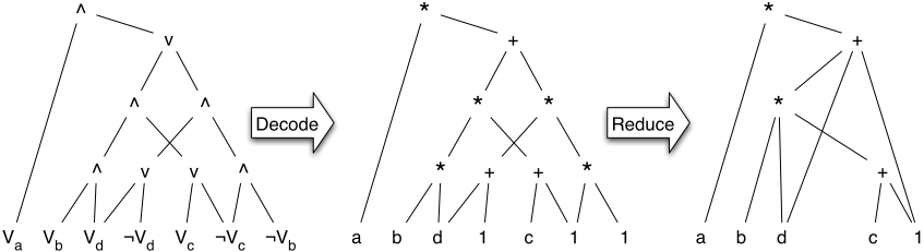
Consider again the CNF ∆f = Va ∧ (Vb ⇒ Vd) ∧ (Vc ⇒ Vb) from the previous section, and the MLF f = a + ad + abd + abcd that it encodes. We now briefly describe the CNF factoring process which allows us to produce the AC shown in Figure 2. First, the output of the factoring process is shown on the left of Figure 3: It is a logical form known as negation normal form (NNF) which satisfies decomposability (conjunctions do not share variables), determinism (disjuncts must be logically incompatible), and smoothness (disjuncts must mention the same sets of variables). Such a factorization is generated using an exhaustive version of the DPLL procedure [Davis et al., 1962]. In particular, the algorithm will pick a variable x in the CNF, will factor ∆|x and ∆|¬x separately, and then combine the results into x ∧ factor(∆|x) ∨ ¬x ∧ factor(∆|¬x). To improve performance, the algorithm keeps a cache that stores CNFs that have been factored and their factorizations and checks this cache before trying to factor a CNF Γ. Finally, before picking a variable x to split Γ on, the algorithm checks the CNF to see if it can be broken into disconnected components, say α1 and α2. In that case, the algorithm factors the components separately and combines their results into factor(α1) ∧ factor(α2). The factoring algorithm we use [Darwiche, 2004], utilizes a decomposition tree (dtree) to manage this decomposition process. In particular, a dtree for a CNF is a binary tree whose leaves correspond to the CNF clauses. Moreover, each node in the dtree is associated with a set of variables whose instantiation is guaranteed to decompose the CNF into two independent components.
The above procedure generates NNFs that are decomposable and deterministic. Smoothness can be established easily by a postprocessing step. Given an NNF that satisfies the required properties, we can extract an AC by simply replacing conjunctions with multiplications, disjunctions with additions, and negative literals with the constant 1. Positive literals are replaced by the real-valued variables they encode. This decoding process is shown in Figure 3; see [Darwiche, 2002] for more details.
This factoring algorithm is indeed a logical version of the recursive conditioning (RC) algorithm [Darwiche, 2001b]. 3
3 Similar algorithms have been used recently to solve probabilis-
| Network | Max Clust | Vars | Card | Ave Card | Total Parms | Max CPT Parms | Ave CPT Parms | %Det | %DP |
|---|---|---|---|---|---|---|---|---|---|
| alarm | 7.2 | 37 | 2-4 | 2.8 | 752 | 108 | 20 | 0.9 | 24.6 |
| bm | 20.0 | 1005 | 2-2 | 2.0 | 6972 | 8 | 7 | 99.6 | 100.0 |
| diabetes | 17.2 | 413 | 3-21 | 11.3 | 461069 | 7056 | 1116 | 78.2 | 17.6 |
| hailfinder | 11.7 | 56 | 2-11 | 4.0 | 3741 | 1188 | 67 | 15.7 | 26.9 |
| mildew | 21.4 | 35 | 3-100 | 17.6 | 547158 | 280000 | 15633 | 93.2 | 25.1 |
| mm | 23.0 | 1220 | 2-2 | 2.0 | 8326 | 8 | 7 | 98.7 | 75.0 |
| munin1 | 26.8 | 189 | 1-21 | 5.3 | 19466 | 600 | 103 | 66.5 | 61.2 |
| munin2 | 18.6 | 1003 | 2-21 | 5.4 | 83920 | 600 | 84 | 63.3 | 69.5 |
| munin3 | 17.8 | 1044 | 1-21 | 5.4 | 85855 | 600 | 82 | 63.1 | 71.3 |
| munin4 | 21.4 | 1041 | 1-21 | 5.4 | 98183 | 600 | 94 | 64.5 | 65.3 |
| pathfinder | 15.0 | 109 | 2-63 | 4.1 | 97851 | 8064 | 898 | 56.1 | 5.1 |
| pigs | 17.4 | 441 | 3-3 | 3.0 | 8427 | 27 | 19 | 56.2 | 23.9 |
| students | 22.0 | 376 | 2-2 | 2.0 | 2616 | 8 | 7 | 90.7 | 79.3 |
| tcc4f | 10.0 | 105 | 2-2 | 2.0 | 3236 | 512 | 31 | 0.4 | 35.6 |
| water | 19.9 | 32 | 3-4 | 3.6 | 13484 | 3072 | 421 | 54.0 | 57.0 |
One can in principle use RC to compile a Bayesian network directly into an AC (bypassing the CNF encoding), but the approach we use allows us to capitalize on the state of the art in logical reasoning for handling determinism and CSI, even though it may incur more overhead in the factoring process. In particular, our CNF factoring algorithm uses unit resolution to propagate logical constraints; conflict directed backtracking to recover more efficiently when conditioning on variable settings that lead to contradictions; in addition to clause learning as a means for avoiding such contradictions early on in future conditioning. It also provides a more flexible framework for exploiting CSI through the use of two techniques. First, it can detect non-structural decompositions, that is, subproblems that become independent due to conditioning on specific variable values-such independence cannot be detected based only on structural considerations (network topology). This is done by removing clauses that become subsumed due to conditioning, therefore, disconnecting subsets of the CNF under specific variable values. Second, it uses a non-structural caching scheme which allows one to prove the equivalence of subproblems under specific variable values (therefore, avoiding multiple factorings of the same subproblem). Again, these equivalences cannot be proven if we were to only use structural considerations. Finally, the re-
tic inference using #SAT [Bacchus et al., 2003].
duction to CNF allows one to more naturally accommodate other types of CPT structures (e.g., decision trees and rules) without the need for algorithmic change. The reduction to CNF factoring and the corresponding techniques lead to quite a bit of overhead in some cases, but this is justified since it will only be done once when compiling the network into an AC. If the application of these techniques lead to smaller ACs, the compile time can then be amortized over all online queries. We will illustrate this benefit more concretely in the experimental results section.
3.2 Encoding parameter equality / CSI
The CPT depicted in Figure 1 has 12 parameters, yet only 5 of these are distinct. Some of the equalities among parameters imply context-specific independence; others do not. For example, the equality between parameters in rows 4 - 6 with those in rows 10-12 imply that C is independent of A given B = b2. However, the equality between parameters in rows 2 and 3 do not imply a CSI.
From a purely encoding viewpoint, one would clearly want to exploit parameter equality, at least to reduce the number of Boolean variables one must generate. Table 2 shows the extent to which parameter equality can help in this regard. In particular, the table reports as %DP the percentage of distinct parameters among non-extreme parameters. That is, the percentage of parameters that would remain if, for each CPT, we collapsed equal, non-extreme parameters into a single parameter. The dramatic example here is pathfinder: about half of its parameters are extreme, and among the other half, only about 5% are distinct within their CPTs. In addition to generating smaller CNFs, encoding parameter equality allows the compiler to run with less overhead, and to generate smaller ACs since parameter equality provides more opportunities for factoring, which immediately translates to gains in online inference.
A key observation here is that no two parameters in the same CPT can ever appear in the same MLF term, as they correspond to incompatible network instantiations. This observation suggests that we can use the same Boolean variable to represent multiple parameters, assuming that such parameters have equal values and appear in the same CPT. However, the idea will not work when applied to PREV. Consider again the CPT in Figure 1. If we use the same variable θ to represent parameters θc2|a1,b1 and θc3|a1,b2 , which are both equal to .5, we would get the following two PI clauses in the CNF: θ ⇒ λb1 and θ ⇒ λb2 , which is inconsistent with other clauses. More generally, PI clauses assert that a parameter implies the corresponding family instantiation. Therefore, if we simply use the same Boolean variable to represent equal parameters, we would be implying inconsistent family instantiations. 4
The solution we adopt is to drop PI clauses from the encoding! Note that dropping PI clauses introduces additional (unintended) models into the CNF, allowing MLF terms which contain multiple parameters from the same CPT. These unintended models/terms, however, can be easily filtered during the decoding process given the following.
Theorem 1 Consider a Bayesian network with n variables. Let ∆ be a CNF encoding which includes the indicator, IP and PI clause sets, and let Γ be the CNF encoding which includes the indicator and IP clause sets only. Then ∆'s models have cardinality 2n and are a subset of Γ's models. Moreover, if σ is a model of Γ but not ∆, then σ's cardinality is > 2n.
Therefore, unintended models have a higher cardinality than original models (which all have the same cardinality). As it turns out, if Γ is an NNF which satisfies decomposability, determinism and smoothness, one can in linear time obtain another NNF Γ′ whose models are exactly the minimum cardinality models of Γ and which satisfies the required properties [Darwiche, 2001a]. Therefore, we can safely drop PI clauses as long we minimize the resulting NNF before we decode the AC.
By including only indicator and IP clauses, we can now safely represent all equal parameters within the same CPT by a single Boolean variable in the CNF encoding. For the Pathfinder network for example, this drops the number of Boolean variables needed to represent non-extreme parameters from 42, 946 to 2, 186, a 95% reduction! Similar reductions are obtained for many other networks; see Table 2. As we show later, not only does this technique improve the compilation time, but can lead to significantly smaller ACs.
4 A restricted case of encoding parameter equality was discussed in [Darwiche, 2002].
3.3 Amore informed factoring algorithm
The CNF factoring algorithm employs two key techniques as discussed earlier. The first is variable splitting, which can be thought of as doing case analysis. The second is caching, so that one can avoid factoring the same CNF subset multiple times. Which variables the algorithm ends up splitting on can very much affect its running time, and the size of factorizations it generates. Moreover, the complexity of the caching scheme is proportional to the number of variables appearing in the cached CNF subset, as the state of such variables are used to generate keys that uniquely define CNFs. The following observations state interesting properties of our CNF encodings, which if passed to the factoring algorithm can significantly improve both the splitting and caching processes.
First, if two clauses share a parameter variable, then they must also share indicators over the same network variable. This property, and the presence of indicator clauses, allow the CNF factoring algorithm to restrict its splitting to indicator variables, which would be sufficient to decompose the problem into independent components (hence, no splitting/case analysis is needed on parameter variables). Second, given the structure of indicator and IP clauses, the state of indicator variables are sufficient to characterize the state of parameter variables. This property allows us to only involve indicator variables when generating CNF keys during the caching process. Both of the above optimizations can be exploited by simply identifying parameter variables to the factoring algorithm.
Another technique that we have used in some of the experiments involves the construction of a decomposition tree (dtree) for the given Bayesian network, and then converting it into a dtree for its CNF encoding. A dtree for a Bayesian network is simply a binary tree whose leaves correspond to the network CPTs [Darwiche, 2001b]. A dtree for a CNF is also a binary tree, but its leaves correspond to the CNF clauses. Since each clause in the CNF encoding is generated by a CPT, we can convert a network dtree into a CNF dtree by simply unfolding the dtree node corresponding to a CPT into a subtree whose leaves correspond to the clauses generated by that CPT. The main point of this technique is to more efficiently generate dtrees for very large CNF encodings that are generated by Bayesian networks with a small number of CPTs (this happens when the network contains very large CPTs).
3.4 Other Optimizations
Our CNF encodings utilize some additional enhancements, two of which are described next. First, we define a new type of clause, called an eclause, which has the same syntax as a regular clause but stronger semantics: it asserts that exactly one of it literals is true. We use eclauses for representing indicator clauses, therefore reducing the size of CNFs considerably in networks having multi-valued variables. Moreover, we outfit the DPLL procedure used in factoring the CNF to work directly with eclauses, without having to unfold them into regular clauses. For another optimization example, the indicators and parameters corresponding to the same state of a root variable are logically equivalent, making it possible to delete the parameter variables and the corresponding IP and PI clauses, which establish the equivalence.
4 Experimental Results
Experiments ran on a 1.6GHz Pentium M with 2GB of RAM, using the networks in Table 2. Two important columns in Table 2 are %Det, which is the percent of parameters that are equal to 0 or to 1 and %DP, which is the percent of nonextreme parameters remaining after collapsing equal parameters within the same CPT. These two values give an idea of the amounts of local structure in the form of determinism and possibly CSI. bm-5-3, mm-3-8-3, and stud-3-2 are networks on which PREV was already shown to perform well by only encoding determinism [Chavira et al., 2004]. These networks contain only binary variables, are highly deterministic, and have small CPTs (no more than two parents per node). In contrast, the other networks contain variables with higher cardinalities and lesser degrees of determinism and, sometimes, very large CPTs. These networks came from various sources: http://www2.sis.pitt.edu/∼genie; Hughes Research Labs; and http://www.cs.huji.ac.il/labs/compbio/Repository.
The experiments serve to demonstrate three points. First, the new CNF encoding and the additional information we pass to the CNF factoring algorithm lead to significant improvement, both in the factoring time and the size of resulting factorizations. Table 4 (1st three columns) illustrates the improvement in factoring time, showing order of magnitude improvements in some cases and allowing us to factor some networks for the first time under the given memory constraints.
The second point illustrated by our experiments concerns the quality of factorizations (ACs) we obtain, compared to the ones embedded in jointrees. Recall that every jointree embeds an AC [Park and Darwiche, 2003], whose size depends only on the jointree size and, hence, is not dependent on local structure. Our experiments are therefore set to illustrate the extent to which local structure can help the factorization process. Table 4 illustrates significant improvements in AC size, as we obtained one to two orders of magnitude improvement on networks such as Water, Pathfinder, Munin1, and Munin4. For a more direct measure of improvement in online inference, 5 we generated sixteen random sets of evidence, and for each evidence set, we computed the marginal of each network variable using jointree propagation and then using AC evaluation/differentiation. 6 Table 4 shows the obtained improvements in online inference, which are similar to improvements in AC size.
Note that since the AC is compiled independently of evidence, the improvements apply for computing all marginals regardless of evidence. This is especially useful for tasks that apply a massive number of queries to Bayesian networks, including parameter estimation algorithms (e.g., EM) given known local structure in the form of determinism and CSI, and MAP algorithms based on branch&bound search.
[Poole and Zhang, 2003] present another approach for exploiting local structure, by providing a refinement on variable elimination (VE). Their approach does not involve a compilation step, and their results are sensitive to the given queries, so a direct comparison between the two approaches is not too meaningful. Yet, we mention here that on a re-parameterized version of Water (to introduce local structure), [Poole and Zhang, 2003] show a factor of 4 improvement over standard VE (total time over all queries; the speedup was more or less depending on the query). Water is the only network from Table 4 that [Poole and Zhang, 2003] report on. Note that the exploitation of local structure can incur overhead that may not be justifiable unless the savings due to local structure are significant enough (not all of the cases in Table 4 lead to significant savings). This appears to be less an of an issue in our approach, since the overhead is pushed into the compilation step. However, in [Poole and Zhang, 2003] which does not involve a compilation step, this overhead is incurred in every query which may or may not lead to overall savings depending on the query-being query specific, however, may sometimes pay off quite significantly, since work performed can sometimes be simplified given specific evidence and specific query variables.
5 Online inference time is affected by the number of AC nodes too (not reported), and by the structure of ACs which affects locality of reference (the ACs embedded in jointrees have better locality).
6 AC differentiation provides more information that just marginals [Darwiche, 2003].
| Local structure | Pathfinder | Water | Munin4 |
|---|---|---|---|
| Det/Equal Parms | 42,810 | 134,140 | 5,762,690 |
| Det only | 130,380 | 138,501 | 9,997,267 |
| Equal Parms only | 200,787 | 11,111,104 | 17,612,036 |
| No local structure | 784,330 | 15,305,634 | - |
| Jointree | 981,178 | 13,777,166 | 116,136,985 |
Our final point regards the effect of local structure on the quality of factorizations. Consider Table 5, which shows AC sizes under different encodings of local structure. First, it is obvious that encoding local structure is responsible for the significant improvements on these networks. Second, in Water, determinism appears to be the main responsible factor. However, in Pathfinder and Munin4, parameter equality alone (without determinism) is sufficient to bring about most of the reported improvements, even though determinism alone can have a similar effect too. Note that there is some overlap between determinism and parameter equality since by encoding determinism (0 parameters), one is effectively collapsing all 0 parameters (applying implicit parameter equality). The results for Pathfinder and Munin4 are therefore not surprising, suggesting possibly that parameter equality is more fundamental than determinism for these networks.
5 Conclusion
We considered the problem of compiling Bayesian networks into ACs. Our aim was to efficiently compile networks having local structure, yet large CPTs and no excessive determinism. We proposed a new encoding scheme that facilitates the representation of local structure in the form of parameter equality, and identified some of its properties that improve compile time. Our results demonstrate significant improvements in both offline/compile and online/inference time, leading to orders of magnitude improvement in online inference.
| Network | Offline Compile Time (s) | AC Edge Count | Online Inference Time (s) | ||||||
|---|---|---|---|---|---|---|---|---|---|
| PREV | NEW | Improv. | Jointree | NEW | Improv. | Jointree | NEW | Improv. | |
| alarm | 0.93 | 0.52 | 1.8 | 4,804 | 2,686 | 1.8 | 0.07 | 0.01 | 6.4 |
| bm-5-3 | 2.51 | 1.11 | 2.3 | 86,532,336 | 18,693 | 4,629.1 | 165.15 | 0.09 | 1,814.8 |
| diabetes | - | 2,269.05 | - | 40,673,307 | 13,585,023 | 3.0 | 37.09 | 16.27 | 2.3 |
| hailfinder | 2.26 | 0.86 | 2.6 | 36,342 | 15,687 | 2.3 | 0.13 | 0.06 | 2.2 |
| mildew | - | 7,483.80 | - | 16,171,408 | 2,123,309 | 7.6 | 13.39 | 3.35 | 4.0 |
| mm-3-8-3 | 7.44 | 1.87 | 4.0 | 98,044,208 | 263,835 | 371.6 | 248.15 | 0.21 | 1,181.6 |
| munin1 | - | 1,534.97 | - | 1,047,211,866 | 30,620,744 | 34.2 | 1,321.68 | 44.91 | 29.4 |
| munin2 | 3,248.42 | 225.46 | 14.4 | 24,281,678 | 4,791,974 | 5.1 | 28.32 | 6.59 | 4.3 |
| munin3 | 1,553.43 | 151.72 | 10.2 | 14,333,412 | 2,436,598 | 5.9 | 18.69 | 3.65 | 5.1 |
| munin4 | 2,440.30 | 677.92 | 3.6 | 116,136,985 | 5,762,690 | 20.2 | 137.94 | 7.70 | 17.9 |
| pathfinder | 226.37 | 20.36 | 11.1 | 981,178 | 43,064 | 22.8 | 1.68 | 0.07 | 23.7 |
| pigs | 110.10 | 17.84 | 6.2 | 2,347,299 | 1,302,215 | 1.8 | 3.45 | 1.60 | 2.2 |
| students-3-2 | 1.53 | 0.82 | 1.9 | 37,799,472 | 27,292 | 1,385.0 | 55.98 | 0.07 | 799.7 |
| tcc4f.obfuscated | 4.11 | 1.15 | 3.6 | 29,064 | 22,284 | 1.3 | 0.14 | 0.05 | 2.8 |
| water | 34.82 | 4.83 | 7.2 | 13,777,166 | 134,142 | 102.7 | 22.68 | 0.21 | 107.5 |
Acknowledgments
We thank the reviewers for commenting on an earlier version of this paper. This work has been partially supported by NSF grant IIS-9988543 and MURI grant N00014-00-1-0617.
@inproceedings{ijcai2005p111,
  title     = {Compiling Bayesian Networks with Local Structure},
  author    = {Chavira, Mark and Darwiche, Adnan},
  booktitle = {Proceedings of the Nineteenth International Joint Conference on
               Artificial Intelligence, {IJCAI-05}},
  publisher = {International Joint Conferences on Artificial Intelligence},
  editor    = {Leslie Pack Kaelbling and Alessandro Saffiotti},
  pages     = {1306--1311},
  year      = {2005},
  url       = {https://ijcai.org/proceedings/2005/111},
}
TY - CPAPER TI - Compiling Bayesian Networks with Local Structure AU - Chavira, Mark AU - Darwiche, Adnan T2 - Proceedings of the Nineteenth International Joint Conference on Artificial Intelligence, IJCAI-05 PB - International Joint Conferences on Artificial Intelligence PY - 2005 SP - 1306 EP - 1311 UR - https://ijcai.org/proceedings/2005/111 ER -Copied
Machine-readable versions of this paper, for tools and AI agents:





