Efficient Reinforcement Learning with Hierarchies of Machines by Leveraging Internal Transitions

1 Introduction

Reinforcement learning (RL) tackles the problem of learning a rewarding behavior in an unknown environment via trial-and-error [Sutton and Barto, 1998]. Recent advances in RL have led to great success on problems that pose significant challenges [Kober and Peters, 2012; Mnih et al., 2015; Silver et al., 2016]. However, standard "flat" RL algorithms often learn slowly in environments requiring complex behaviors, due to the curses of dimensionality and history. Hierarchical reinforcement learning (HRL) aims to scale RL by incorporating prior knowledge about the structure of good policies into the algorithms [Barto and Mahadevan, 2003]. Popular HRL solutions include the options theory [Sutton et al., 1999], the hierarchies of abstract machines (HAMs) framework [Parr and Russell, 1998; Andre and Russell, 2001], and the MAXQ approach [Dietterich, 1999]. One of the major advantages of HRL approaches is the possibility of exploiting temporal abstraction and hierarchical control, where macroactions following their own polices until termination.

This paper describes a new HRL algorithm taking advantage of internal transitions introduced by the input hierarchical structure, following the framework of HAMs. The idea of HAMs is to write a partial policy for an agent, and use RL to learn its optimal completion. A partial policy (or a HAM

Stuart Russell

UC Berkeley russell@cs.berkeley.edu

hereinafter) can be represented as a set of hierarchical finite state machines (FSMs), with unspecified choice states. To run a HAM, a run-time stack is needed to maintain the complete machine state. An agent equipped with a HAM interacting with its environment reduces to a semi Markov decision process (SMDP) defined over the joint space of environment and machine states. A choice point is defined as a joint state with the top of the stack being a choice state. Learning happening at choice points suffices to find an optimal policy for the resulting SMDP, which corresponds to the optimal completion of the HAM. Comparing with options and MAXQ, the main advantages of HAMs are that it encodes complex behaviors with arbitrary hierarchical structure, it supports passing parameters and storing local variables within the run-time stack, and it enables learning of an optimal hierarchical policy consistent with the input hierarchical structure.

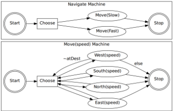
It is our observation that a HAM with deep hierarchical structure, where there are many calls from a parent machine to one of its child machines over the hierarchy, induces many internal transitions. An internal transition is a transition over the joint state space, where only the run-time stack changes but the environment state does not. Internal transitions always come with zero rewards and deterministic outcomes in the resulting SMDP. For an example, see Figure 1, which shows a HAM for a mobile robot navigating in a grid map. The Navigate machine has a choice state, at which it has to choose between Move(Fast) and Move(Slow). The Move(speed) machine has to select repeatedly between East, West, South and North with specified speed parameter until the robot is at its destination. In this simple example, if the choice made at stack [Navigate, Choose] is Move(Fast), then the stack of the next choice point must be [Navigate, Choose, Move(Fast), Choose]. It is not uncommon that there could be many such internal transitions in a HAM with arbitrary structure for a complex domain. It is actually easier for a human designer to come up with a deep HAM, rather than a shallow HAM. In the setting of concurrent learning when multiple HAMs are running concurrently, as shown in [Marthi et al., 2005], there are even more opportunities to have internal transitions defined over the resulting joint SMDP.

In this paper, we present HAMQ-INT, a HAMQ-based HRL algorithm that identifies and exploits internal transitions within a HAM for efficient learning. HAMQ-INT recursively shortcircuits the computation of Q values whenever applicable. We empirically confirm that HAMQ-INT outperforms the state of the art significantly on the benchmark Taxi domain and a much more complex RoboCup Keepaway domain. The two contributions of this paper is that 1) we develop the novel HAMQ-INT algorithm, and 2) we apply it successfully to the RoboCup Keepaway domain, which, to the best of our knowledge, is the first application of the HAM framework to a very complex domain.

The paper is organized as follows. Section 2 briefly introduces some background on Markov decision processes and reinforcement learning. Section 3 introduces the fundamental HAM framework. Section 4.1 presents the main results, and Section 4.2 details the HAMQ-INT algorithms - efficient HAM learning by leveraging internal transitions. Section 5 describes the empirical results on Taxi and RoboCup Keepaway domains. In Section 6, we conclude with discussion of future work.

2 Background

Markov decision processes (MDPs) provide a rich framework for planning and learning under uncertainty. Formally, an MDP is a tuple 〈S,A, T,R, γ〉, where S and A are the state and action spaces, T(s′ |s, a) and R(s, a) are the transition and reward functions, and γ is a discount factor [Bellman, 1957]. The goal for an MDP is to find an optimal policy π∗ : S → A that maximizes the expected cumulative reward. In the setting of reinforcement learning, an agent learns an optimal policy by interacting with its environment. A Q learning agent achieves this by performing Q update, once it reaches state s′ with reward r after executing action a in state s:

where α is a learning rate.

Semi Markov decision processes (SMDPs) allow for actions that take multiple time steps to terminate. The transition function for an SMDP has the form T(s′ ,N|s, a), where N is the number of time steps that action a takes. Similarly, the Q update rule for a SMDP is:

where τ is number of time steps elapsed after executing action a in state s and before reaching state s′ , and r is the cumulative reward in-between.

Run(N : machine, z : stack, s : environment state): z.Push(N) m ← N .start while m ̸= N .stop do if Type(m) = action then s ← Execute(µ(m)) else if Type(m) = call then s ←Run(µ(m), z, s, π) if Type(m) = choose then z.Push(m) m←Choose(z, s, µ(m)) z.Pop() elsem ← δ(m, s) z.Pop() return s

3 The HAMFramework

The idea of HAM is to encode a partial policy for an agent as a set of hierarchical finite state machines with unspecified choice states, and use RL to learn its optimal completion. We adopt a different definition of HAM, allowing arbitrary call graph, despite the original definition of Parr and Russell [1998] which requires that the call graph is a tree. Formally, a HAM H = {N0,N1, . . . } consists of a set of Moore machines Ni [Moore, 1956], where N0 is the root machine which serves as the starting point of the agent. A machine N is a tuple 〈M, Σ, Λ, δ, µ〉, where M is the set of machine states, Σ is the input alphabet which corresponds to the environment state space S, Λ is the output alphabet, δ is the machine transition function with δ(m, s) being the next machine state given machine state m ∈ M and environment state s ∈ S, and µ is the machine output function with µ(m) ∈ Λ being the output of machine state m ∈ M. There are 5 types of machine states: start states are the entries of running machines; action states execute an action in the environment; choose states nondeterministically select the next machine states; call states invoke the execution of other machines; and, stop states end current machines and return control to calling machines. A machine N has uniquely one start state and one stop state, referred as N.start and N.stop respectively. For start and stop states, the outputs are not defined; for action states, the outputs are the associated primitive actions; for call states, the outputs are the next machines to run; and, for choose states, the outputs are the sets of possible choices, where each choice corresponds to a next machine state.

To run a HAM H, a run-time stack (or stack for short) is needed. Each frame of this stack stores run-time information such as the active machine, its machine state, the parameters passing to this machine and the values of local variables used by this machine. Algorithm 1 gives the pseudo-code for running a HAM, where the Execute function executes an action in the environment and returns the next environment state, and the Choose function picks the next machine state given the updated stack z, the current environment state s

Navigate(s : environment state): speed ← Choose1(Slow, F ast) s ← Move(s, speed) return s Move(s : environment state, speed : parameter): while not s.atDest() do a ← Choose2(West, South, North, East) s ← Execute(a, speed) return s

and the set of available choices µ(m). Let Z be the space of all possible stacks given HAMH. It has been shown that an agent running a HAM H over an MDP M yields a joint SMDP H ◦M defined over the joint space of S and Z. The only actions of H ◦ M are the choices allowed at choice points. A choice point is a joint state (s, z) with z.Top() being a choose state. This is an SMDP because once a choice is made at a choice point, the system - the composition of H and M- runs automatically until the next choice point is reached. The policy of this SMDP implements exactly the Choose function in Algorithm 1. An optimal policy of this SMDP corresponds to an optimal completion of the input HAM, which can be found by applying a HAMQ algorithm [Parr and Russell, 1998]. HAMQ keeps track of the previous choice point (s, z), the choice made c and the cumulative reward r thereafter. Whenever it enters into a new choice point (s′ , z′ ), it performs the SMDP Q update as follows:

where τ is the number of steps between the two choice points. As suggested by the language of ALisp [Andre and Russell, 2002], a HAM can be equivalently converted into a piece of code in modern programming languages, with call-andreturn semantics and built-in routines for explicitly updating stacks, executing actions and getting new environment states. The execution of a HAM can then be simulated by running the code itself. This conversion is important, as it provides a much more efficient way of designing and running a HAM. For example, the HAM shown in Figure 1 is equivalent to the pseudo-code in Algorithm 2, where a machine becomes a function. Here, Execute is the macro executing an action with specified parameters and returning the next environment state; the Choose macro extends the Choose function from Algorithm 1 to choose among not only a set of machine states, but also a set of parameters for the next machine. Bookkeeping codes for maintaining the stack are omitted for simplicity.

4 The Main Approach

This section presents the main approach. We first introduce internal transitions within HAMs, and then develop an algorithm that automatically discovers and take advantage of internal transitions for fast learning.

4.1 Internal Transitions within HAMs

In general, the transition function of the resulting SMDP induced by running a HAM has the form T(s′ , z′ , τ|s, z, c) ∈

[0, 1], where (s, z) is the current choice point, c is the choice made, (s′ , z′ ) is the next choice point, and τ is the number of time steps. Given a HAM with a deep hierarchy of machines, it is usually the case that there is no real actions executed between two consecutive choice points, therefore the number of time steps and the cumulative reward in-between are essentially zero. We call this kind of transition an internal transition, because the machine state changes but the environment state does not. Formally, a transition is a tuple 〈s, z, c, r, s′ , z′ 〉 with r being the cumulative reward. For an internal transition, we must have s′ = s and r = 0. In addition, because the dynamics of the HAM after a choice has been made and before an action is executed is deterministic by design, the next choice point (s, z′ ) of an internal transition is deterministically conditioned only on 〈s, z, c〉. Let ρ(s, z, c) be the Z component of the next choice point. If 〈s, z, c〉 leads to an internal transition, we must have T (s, ρ(s, z, c), 0|s, z, c) = 1. Therefore, we have

So, we can store the rules of internal transition as 〈s, z, c, z ′ 〉 tuples, where z′ = ρ(s, z, c). They can be used to recursively compute Q values according to Equation 3 when applicable. The size of the set of stored rules can be further reduced, because the machine transition function δ of a HAM is usually determined by a set of predicates defined over environment state s, rather than the exact values of all state variables. For example, the machine transition function of machine Move(speed) in Figure 1 depends only on the value of atDest(s) for any state s. Suppose 〈s1, z, c〉 leads to an internal transition with (s1, z′ ) being the next choice point. Let the set of predicates used to determine the trajectory in terms of active machines and machine states from z.Top() to z′ .Top() be P = {P1, P2, . . . }. Let the value of P given state s be P(s) = {P1(s), P2(s), . . . }. It can be concluded that the transition trajectory induced by P depends only on P(s1), after choice c is made at choice point (s1, z). On the other hand, if the set of predicates P over state s2 (s2 ̸= s1) has the same value as of state s1, namely P(s2) = P(s1), and the same choice c is made at choice point (s2, z), then the followed transition trajectory before reaching the next choice point must also be the same as of 〈s1, z, c〉. In other words, 〈s2, z, c〉 leads to an internal transition such that ρ(s1, z, c) = ρ(s2, z, c).

Thus, the rule of internal transition 〈s1, z, c, z ′ 〉 can be equivalently stored and retrieved as 〈P,P(s1), z, c, z ′ 〉, which automatically applies to 〈s2, z, c, z ′ 〉, if P(s2) = P(s1). Here, z′ is the stack of the next choice point such that z′ = ρ(s1, z, c) = ρ(s2, z, c). The size of the joint space of encountered predicates and their values is determined by the HAM itself, which is typically much smaller than the size of the state space. For example, for a problem with continuous state space (such as the RoboCup Keepaway domain we considered), this joint space is still limited. In summary, we can have an efficient way of storing and retrieving the rules of internal transition by keeping track of the predicates evaluated between two choice points.

4.2 The HAMQ-INT Algorithm

The idea of HAMQ-INT is to identify and take advantage of internal transitions within a HAM. For this purpose, HAMQINT automatically keeps track of the predicates that are evaluated between two choice points, stores the discovered rules of internal transition based on predicates and the corresponding values, and uses the learned rules to shortcircuit the computation of Q values whenever it is possible. To detect internal transitions, a global environment time t is maintained. It is incremented by one only when there is an action executed in the environment. When the agent enters a choice point (s′ , z′ ) after having made a choice c at choice point (s, z), and finds that t is not incremented since the previous choice point, it must be the case that s′ = s and 〈s, z, c〉 leads to an internal transition. Let P be the set of predicates that have been evaluated between these two choice points. Then a new rule of internal transition 〈P,P(s), z, c, z ′ 〉 is found. The agent can conclude that for any state x, if P(x) = P(s), then 〈x, z, c〉 leads to an internal transition as well. In the implementation, the agent uses a hash table ρ to store the learned rules, such that ρ[P,P(s), z, c] = z′ , if 〈P,P(s), z, c, z ′ 〉 is a rule of internal transition. One thing to note is that, because z′ is deterministically conditioned on 〈P,P(s), z, c〉 for an internal transition, the value of ρ[P,P(s), z, c] will not be changed after it has been updated for the first time.

When the agent needs to evaluate a Q function, say Q(s, z, c), and finds that 〈s, z, c〉 leads to an internal transition according to the current learned rules, Equation 3 is used to decompose Q(s, z, c) into the Q values of the next choice points, which are evaluated recursively in the same way, essentially leading to a tree of exact Bellman backups. In fact, only the terminal Q values of this tree needs to be learned, enabling efficient learning for the agent. Algorithm 3 gives the pseudo-code of the HAMQ-INT algorithm. Here, the QTable function returns the stored Q value as request. It can be implemented in either tabular or function approximation ways. The Q function evaluates the Q value of (s, z, c) tuple. It first checks whether (s, z, c) subjects to any learned internal transition rule. This is done by checking whether there exists an encountered set of predicates P, such that 〈P,P(s), z, c〉 ∈ ρ.Keys(). The uniqueness of transition trajectory for an internal transition ensures that there will be at most one such P. If there is such P, Q uses the retrieved rule to recursively decompose the requested Q value according to Equation 3; otherwise, it simply returns the stored Q value by querying QTable.

The QUpdate function performs the SMDP Q update. It is called once the agent enters a new choice point. The caller has to keep track of the current state s′ , the current stack z′ , the evaluated predicates P on state since the previous choice point and the cumulative reward r in-between. If the current time t′ equals to the time t of the previous choice point, it must be the case that 〈s, z, c, 0, s, z ′ 〉 is an internal transition. Thus, a new rule 〈P,P(s), z, c〉 is learned, and the ρ table is updated accordingly. If t′ ̸= t, meaning there are some actions executed in the environment, it simply performs the Q update. Finally, it uses the current (t′ , s′ , z′ ) tuple to update the (global) previous (t, s, z) tuple, so the function will be prepared for the next call.

QUpdate(s′ : state, z′ : stack, r : reward, t′ : current time, P : evaluated predicates): if t′ = t then ρ[P, P(s), z, c] ← z′ else QTable(s, z, c) ← (1 - α) QTable(s, z, c) +α(r + γ t′-t maxc′ Q(s′ , z′ , c′) ) (t, s, z) ← (t′ , s′ , z′ ) Q(s : state, z : stack, c : choice): if ∃P s.t. 〈P, P(s), z, c〉 ∈ ρ.Keys() then q ← -∞ z′ ← ρ[P, P(s), z, c] for c′ ∈ µ(z.Top()) do q ← max(q, Q(s, z′ , c′) ) return q else return QTable(s, z, c)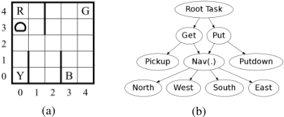

5 Experiments

We conduct experiments on the benchmark Taxi domain [Dietterich, 1999] and a much more complex RoboCup Keepaway domain [Stone et al., 2005]. For all learning algorithms, the learning rate is set to be 0.125; an ϵ-Greedy policy which selects a random action with probability 0.01 is used to balance between exploration and exploitation.

5.1 The Taxi Domain

On the Taxi domain, a taxi navigates in a grid map to pick up and deliver a passenger. In the beginning of each episode, the passenger's initial location and her destination are randomly selected from the 4 terminals: R, G, Y and B. There are 6 primitive actions for the taxi: a) 4 navigation actions: North, West, South and East; b) the Pickup action; and c) the Putdown action. Each navigation action has probability 0.2 of moving into perpendicular directions. At each time step, unsuccessful Pickup and Putdown have a reward of - 10, successful Putdown has a reward of 20, and all other actions have a reward of -1. Algorithm 4 shows the HAM written in pseudo-code for this experiment, where the Root machine repeatedly selects between Get and Put machines until termination; the Get and Put machines are encoded to navigate to the passenger or destination locations first, and then execute Pickup or Putdown actions accordingly; the

Root(s : environment state): while not s.Terminate() do m ← Choose1(Get, Put) s ← Run(m, s) return s Get(s : environment state): s ← Navigate(s, s.Passenger()) s ←Execute(Pickup, s) return s Put(s : environment state): s ← Navigate(s, s.Destination()) s ←Execute(Putdown, s) return s Navigate(s : environment state, w : target): while s.Taxi() ̸= w do m ← Choose2(North, East, South, West) n ← Choose3(1, 2) for i ∈ [1, n] do s ← Execute(m, s) return s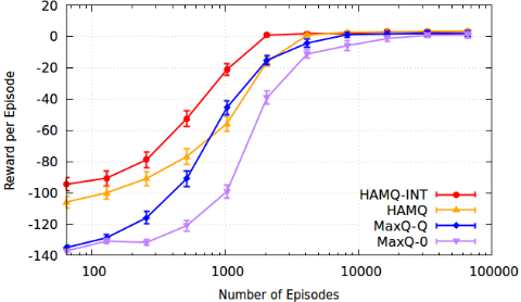

Navigate machine repeatedly selects among the four navigation actions until the taxi reaches its target. It is worth noting that Choose3 is used for encouraging the discovery of temporally-extended action and creating more opportunities for internal transitions. The internal transition happens after a choice is made within the Root machine. For example, when a Get machine is selected at the choice point Choose1 within the Root machine, the next choice point must be Choose2 within the Navigation machine.

We compare HAMQ-INT with HAMQ, MAXQ-0 and MAXQ-Q algorithms. The MAXQ task graph used for MAXQ-0 and MAXQ-Q is shown in Figure 2b. MAXQ-Q is additionally encoded with a pseudo-reward function for the Navigation sub-task, which gives a reward of 1 when terminated. Comparing with MAXQ algorithms, one advantage of HAM is that the Get and Put machines are encoded with the right order of calling other machines, while MAXQ algorithms have to learn this order by themselves. Figure 3 shows the experimental result averaged over 400 runs. It can be seen from the result that MAXQ-Q outperforms MAXQ-0 as expected, HAMQ outperforms MAXQ-Q at the early stage of learning, and HAMQ-INT outperforms HAMQ significantly.

5.2 The RoboCup Keepaway Domain

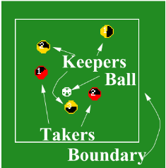
The RoboCup Keepaway problem is a sub-task of RoboCup soccer simulation 2D challenge [Stone et al., 2005]. In Keepaway, a team of keepers tries to maintain the ball possession within a limited field, while a team of takers tries to take the ball. Figure 4 shows an instance of Keepaway with 3 keepers and 2 takers. The system has continuous state and action spaces. A state encodes positions and velocities for the ball and all players. At each time step (within 100 ms), a player can execute a parametrized primitive action, such as turn(angle), dash(power) or kick(power, angle), where the turn action changes the body angle of the player, the dash action gives an acceleration to the player, and the kick action gives an acceleration to the ball if the ball is within the maximal kickable area of the player. All primitive actions are exposed to noises. Each episode begins with the ball and all players at fixed positions, and ends if any taker kicks the ball, or the ball is out of the field. The cumulative reward for the keepers is the total number of time steps for an episode. Instead of learning to select between primitive actions, the players are provided with a set of programmed options including: 1) Stay() remaining stationary at the current position; 2) Move(d, v) dashing towards direction d with speed v; 3) Intercept() intercepting the ball; 4) Pass(k, v) passing the ball to teammate k with speed v; and 5) Hold() remaining stationary while keeping the ball kickable.

In our experiments, the taker is executing a fixed policy, namely it holds the ball if the ball is kickable, otherwise it tries to intercept the ball. This policy is commonly used in the literature. The goal in RoboCup Keepaway is then to learn a best-response policy for the keepers given fixed takers. We develop a HAM policy from the perspective of a single keeper, and run multiple instances of this HAM concurrently for each keeper to form a joint policy for all keepers. To run multiple HAMs concurrently, they have to be synchronized, such that if any machine is at its choose state, the other machines have to wait; if multiple machines are at their choose states, a joint choice is made instead of inde-

Keeper(s : environment state): while not s.Terminate() do if s.BallKickable() then m ← Choose1(Pass, Hold) s ← Run(m, s) else if s.FastestToBall() then s ← Intercept(s) elsem ← Choose2(Stay, Move) s ← Run(m, s) return s Pass(s : environment state): k ←Choose3(1, 2, . . . ) v ← Choose4(Normal, Fast) while s.BallKickable() do s ← Run(Pass, k, v) return s Hold(s : environment state): s ← Run(Hold) return s Intercept(s : environment state): s ← Run(Intercept) return s Stay(s : environment state): i ← s.TmControlBall() while i = s.TmControlBall() do s ←Run(Stay) return s Move(s : environment state): d ←Choose5(0◦ , 90◦ , 180◦ , 270◦) v ← Choose6(Normal, Fast) i ← s.TmControlBall() while i = s.TmControlBall() do v ←Run(Move, d, v) return s

pendent choice for each machine. For this purpose, players have to share their learned value functions and the selected joint choice. A joint Q update is developed to learn the joint choice selection policy as an optimal completion of the resulting joint HAM. Algorithm 5 shows the HAM written in pseudo-code for a single keeper. Here, Keeper is the root machine. The Run macro runs a machine or an option with specified parameters. BallKickable, FastestToBall, TmControlBall are predicates used to determine the transition inside a machine. It is worth noting that the Move machine only considers 4 directions, with direction 0◦ being the direction towards the ball, and so on. There are many internal transitions within this single HAM. For example, when the Pass machine is selected at the choice point Choose1 of the Keeper machine, the next 2 consecutive choice points must be Choose3 and Choose4 within the the Pass machine. When multiple HAMs are executing concurrently, there are even more internal transitions in the resulting joint HAM. For example, in a scenario of the 3 vs. 2 Keepaway game, where only keeper 1 can kick the ball, suppose the joint machine state is [Choose1, Choose2, Choose2] with each element being the machine state of a HAM. If the joint choice made is [Pass, Move, Stay], then the next 2 consecutive machine states must be [Choose3, Choose5, Stay] and [Choose4, Choose6, Stay] following the joint HAM.

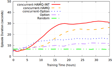
We compare concurrent-HAMQ-INT, concurrent-HAMQ, concurrent-Option, Option and Random algorithms. The Option algorithm is adopted from [Stone et al., 2005], where the agent learns an option-selection policy over Hold() and Pass(k, v) options if it can kick the ball, otherwise it follows a fixed policy: if it is the fastest one to intercept the ball, it intercepts; otherwise, it follows a GetOpen() option. The GetOpen() option, which enables the agent to move to an open area in the field, is manually programmed beforehand. In the original Option learning algorithm, each agent learns independently. We argue that this setting is problematic, since it actually incorrectly assumes that other keepers are stationary. We extend Option to concurrent-Option, by sharing the learned value functions and the option selected. The HAM algorithms are not provided with the GetOpen() option. Instead, they have to learn their own versions of GetOpen() by selecting from Stay and Move machines. The SARSAlearning rule with a linear function approximator (namely tile coding) is used to implement the SMDP Q update for all learning algorithms. The Random algorithm is a non-learning version of Option, which selects available options randomly as a baseline. Figure 5 shows the experiment result on a 3 vs. 2 instance of RoboCup Keepaway averaged using a moving window with size of 1000 episodes. It can be seen from the result that concurrent-Option outperforms Option significantly, concurrent-HAMQ outperforms concurrent-Option after about 15 hours of training, and concurrent-HAMQ-INT has the best performance.

6 Conclusion

In this paper, we present a novel HAMQ-INT algorithm which automatically discovers and exploits internal transitions within a HAM for efficient learning. We empirically confirm that HAMQ-INT outperforms the state of the art significantly on the benchmark Taxi domain and a much more complex RoboCup Keepaway domain. The way we taking advantage of internal transitions within a HAM can be seen as leveraging some prior knowledge on the transition model of a reinforcement learning problem, which happens to have some deterministic transitions. In future work, we would like to extend this idea to more general reinforcement learning problems, where models are partially known in advance.

Acknowledgments

Funding for this research was provided by ONR under contract N00014-12-1-0609, and by DARPA under contract N66001-15-2-4048. Opinions, findings, and conclusion or recommendations expressed in this material are those of the authors and do not necessarily reflect the view of the funding agencies. The authors would like to thank the anonymous reviewers for their valuable comments and suggestions.