
Dominance and Optimisation Based on Scale-Invariant Maximum Margin Preference Learning
Proceedings of the Twenty-Sixth International Joint Conference on Artificial Intelligence. Main track. Pages 1209-1215.
https://doi.org/10.24963/ijcai.2017/168
Keywords
- Knowledge Representation, Reasoning, and Logic: Preferences
- Uncertainty in AI: Uncertainty in AI
- Machine Learning: Learning Preferences or Rankings
- Knowledge Representation, Reasoning, and Logic: Preference modelling and preference-based reasoning
Abstract
In the task of preference learning, there can be natural invariance properties that one might often expect a method to satisfy. These include (i) invariance to scaling of a pair of alternatives, e.g., replacing a pair (a,b) by (2a,2b); and (ii) invariance to rescaling of features across all alternatives. Maximum margin learning approaches satisfy such invariance properties for pairs of test vectors, but not for the preference input pairs, i.e., scaling the inputs in a different way could result in a different preference relation. In this paper we define and analyse more cautious preference relations that are invariant to the scaling of features, or inputs, or both simultaneously; this leads to computational methods for testing dominance with respect to the induced relations, and for generating optimal solutions among a set of alternatives. In our experiments, we compare the relations and their associated optimality sets based on their decisiveness, computation time and cardinality of the optimal set. We also discuss connections with imprecise probability.
- [Augustin et al., 2014] Thomas Augustin, Frank PA Coolen, Gert de Cooman, and Matthias CM Troffaes. Introduction to Imprecise Probabilities. John Wiley and Sons, 2014.
- [Ben-Hur and Weston, 2010] Asa Ben-Hur and Jason We- ston. A users guide to support vector machines. Data min- ing techniques for the life sciences, pages 223-239, 2010.
- [Birlutiu et al., 2010] Adriana Birlutiu, Perry Groot, and Tom Heskes. Multi-task preference learning with an ap- plication to hearing aid personalization. Neurocomputing, 73(7):1177-1185, 2010.
- [Burges, 1998] Christopher JC Burges. A tutorial on support vector machines for pattern recognition. Data mining and knowledge discovery, 2(2):121-167, 1998.
- [Cortes and Vapnik, 1995] Corinna Cortes and Vladimir Vapnik. Support-vector networks. Machine learning, 20(3):273-297, 1995.
- [Fürnkranz and Hüllermeier, 2010] Johannes Fürnkranz and Eyke Hüllermeier. Preference learning. Springer, 2010.
- [Greco et al., 2010] Salvatore Greco, Vincent Mousseau, and Roman Slowinski. Multiple criteria sorting with a set of additive value functions. European Journal of Opera- tional Research, 207(3):1455-1470, 2010.
- [Herbrich et al., 1999] Ralf Herbrich, Thore Graepel, and Klaus Obermayer. Support vector learning for ordinal re- gression. 1999.
- [Joachims, 2002] Thorsten Joachims. Optimizing search en- gines using clickthrough data. In Proceedings of the eighth ACM SIGKDD international conference on Knowledge discovery and data mining, pages 133-142. ACM, 2002.
- [Kazawa et al., 2005] Hideto Kazawa, Tsutomu Hirao, and Eisaku Maeda. Order SVM: a kernel method for order learning based on generalized order statistics. Systems and Computers in Japan, 36(1):35-43, 2005.
- [Kohli and Jedidi, 2007] Rajeev Kohli and Kamel Jedidi. Representation and inference of lexicographic preference models and their variants. Marketing Science, 26(3):380- 399, 2007.
- [Marinescu et al., 2013] Radu Marinescu, Abdul Razak, and Nic Wilson. Multi-objective constraint optimization with tradeoffs. In International Conference on Principles and Practice of Constraint Programming, pages 497-512. Springer, 2013.
- [Montazery and Wilson, 2016] Mojtaba Montazery and Nic Wilson. Learning user preferences in matching for ridesharing. In Proceedings of the 8th International Con- ference on Agents and Artificial Intelligence (ICAART 2016), volume 2, pages 63-73, 2016.
- [Nilsson, 1986] Nils J. Nilsson. Probabilistic logic. Artif. Intell., 28(1):71-87, 1986.
- [Rossi et al., 2011] Francesca Rossi, Kristen Brent Venable, and Toby Walsh. A short introduction to preferences: be- tween artificial intelligence and social choice. Synthesis Lectures on Artificial Intelligence and Machine Learning, 5(4):1-102, 2011.
- [Stolcke et al., 2008] Andreas Stolcke, Sachin Kajarekar, and Luciana Ferrer. Nonparametric feature normalization for SVM-based speaker verification. In Proceedings of the IEEE International Conference on Acoustics, Speech, and Signal Processing, ICASSP 2008, March 30 -April 4, 2008, Caesars Palace, Las Vegas, Nevada, USA, pages 1577-1580. IEEE, 2008.
- [Trabelsi et al., 2011] Walid Trabelsi, Nic Wilson, Derek Bridge, and Francesco Ricci. Preference dominance rea- soning for conversational recommender systems: a com- parison between a comparative preferences and a sum of weights approach. International Journal on Artificial In- telligence Tools, 20(4):591-616, 2011.
- [Walley, 1991] Peter Walley. Statistical Reasoning with Im- precise Probabilities. Chapman and Hall, London, 1991.
- [Walley, 1996] Peter Walley. Measures of uncertainty in ex- pert systems. Artif. Intell., 83(1):1-58, 1996.
- [Wilson and Montazery, 2016] Nic Wilson and Mojtaba Montazery. Preference inference through rescaling pref- erence learning. In Proceedings of the Twenty-Fifth Inter- national Joint Conference on Artificial Intelligence, IJCAI 2016, New York, NY, USA, 9-15 July 2016, pages 2203- 2209. IJCAI/AAAI Press, 2016. IJCAI
- [Wilson et al., 2015a] Nic Wilson, Anne-Marie George, and Barry O'Sullivan. Computation and complexity of prefer- ence inference based on hierarchical models. In Proceed- ings of the Twenty-Fourth International Joint Conference on Artificial Intelligence, IJCAI 2015, Buenos Aires, Ar- gentina, July 25-31, 2015, pages 3271-3277, 2015. IJCAI
- [Wilson et al., 2015b] Nic Wilson, Abdul Razak, and Radu Marinescu. Computing possibly optimal solutions for multi-objective constraint optimisation with tradeoffs. In Proceedings of the Twenty-Fourth International Joint Con- ference on Artificial Intelligence, IJCAI'15, pages 815- 821. AAAI Press, 2015. IJCAI
- [Xia and Conitzer, 2008] Lirong Xia and Vincent Conitzer. Determining possible and necessary winners under com- mon voting rules given partial orders. In Proceedings of the Twenty-Third AAAI Conference on Artificial Intel- ligence, AAAI 2008, Chicago, Illinois, USA, July 13-17, 2008, volume 8, pages 196-201, 2008.
- [Yannakakis et al., 2009] Georgios N Yannakakis, Manolis Maragoudakis, and John Hallam. Preference learning for cognitive modeling: a case study on entertainment preferences. IEEE Transactions on Systems, Man, and Cybernetics-Part A: Systems and Humans, 39(6):1165- 1175, 2009.
References were extracted automatically from the PDF and may contain errors.
Full text extracted automatically from the PDF; figures, tables and equations may differ. The PDF is the version of record.
1 Introduction
There is a growing trend towards personalisation for services in many real-world application domains, such as ecommerce, marketing, and entertainment. This involves capturing user preferences over alternative choices, e.g., products, movies and hotels. One may view this as an enhanced variation of supervised learning, known as preference learning, where instead of tagging an instance with a single label, preference relations are expressed over instances [Yannakakis et al., 2009; Birlutiu et al., 2010]. These state that one alternative a is preferred over another one b, where an alternative is associated with a feature vector, i.e., a vector of values for a number of features.
An established approach to modeling preferences makes use of the concept of a utility function which is learnt from preference input pairs. Then, for a pair of test vectors (α, β), this function assigns an abstract degree of utility to each test vector, implying which test vector is preferred to which [F¨urnkranz and H¨ullermeier, 2010]. Support Vector Machine (SVM) approaches [Burges, 1998] have inspired the development of several methods for learning the utility function, such as OrderSVM [Kazawa et al., 2005], SVOR [Herbrich et al., 1999] and SVMRank [Joachims, 2002].
In a method such as SVMRank, when the utility function has been learnt, rescaling a pair of test vectors makes no difference to the result, i.e., α is preferred to β if and only if rα is preferred to rβ for any strictly positive scale factor r. The same does not hold for the input pairs: different ways of scaling preference input pairs may lead to a very different utility function being learnt. However, it is arguable that in many contexts, a preference for a over b can be considered as conveying essentially equivalent information to a preference for ra over rb. For instance, knowing that the movie with feature vector a is preferred to one with feature vector b, we would often expect that 2a is preferred to 2b. This suggests defining a more cautious preference relation by saying that a test vector α is preferred to β if α is preferred to β for all choices of scalings of preference input pairs.
An analogous form of preference relation, which is characterised in [Wilson and Montazery, 2016], considers the scaling of features. Part of the motivation for this is that feature scaling is an essential preprocessing phase for any SVMbased method; the scaling, and therefore the resulting preference relation, can sometimes depend strongly on precisely which preference inputs are received.
Taking into account both forms of rescaling mentioned above, we also define a still more cautious relation in which α is preferred to β if it is preferred for all choices of scalings of features and preference input pairs.
Other forms of preference inference, based on more qualitative, lexicographic, models are considered in [Trabelsi et al., 2011; Kohli and Jedidi, 2007; Wilson et al., 2015a]. Other preference reasoning techniques based on a family of utility functions include e.g., [Greco et al., 2010].
The rest of the paper is organised as follows. We explain the maximum margin preference relation in Section 2. Section 3 defines and characterises a preference relation that is invariant to the scaling of preference input pairs in the maximum margin relation. Similarly, the two other relations, where features are rescaled and where both features and preference inputs are rescaled, are characterised in Section 4. The characterisations lead to the computational methods in Section 5. In Section 6, we consider two different notions of optimality for each preference approach, and we report the experimental results in Section 7, comparing the computation time for each relation as well as the number of optimal solutions found according to the two kinds of optimality operator. Section 8 concludes, with a discussion of potential extensions, and of the relationship with imprecise probability. 1
2 MaximumMargin Preference Relation
We first describe a simple linear SVM-based preference relation based on Ranking SVM (or SVMRank) [Joachims, 2002], but only considering consistent inputs.
We assume that some user has told us that he prefers feature vector ai ∈ IRn over bi ∈ IRn , for each i ∈ I = {1, . . . ,m}. Each tuple ai or bi in IRn represents an alternative that is characterised by n features, with e.g., ai(k) being the score for alternative ai regarding the kth feature. 2 By assuming a linear weighting model, each pair (ai, bi) expresses a linear restriction ai ·w > bi ·w on an unknown weight vector w ∈ IRn (the dot product ai · w is equal to ∑nj=1 ai(j)w(j)). This linear weighting assumption is less restrictive than it sounds; for instance, we could form additional features representing e.g., pairwise products of the basic features, enabling a richer representation of the utility function.
We define Λ, the preference inputs, to be {λi : i ∈ I}, where for each i, λi = ai - bi. Then, a feasible w satisfies λ · w > 0 for all λ ∈ Λ (because ai · w > bi · w). We can associate the hyperplane Hw = {x ∈ IRn : x · w = 0} with a feasible w. Clearly, any feasible hyperplane contains the origin, and all λ ∈ Λ are in the associated positive open half-space.
Example 1. Suppose that n = 2 and let the preference inputs Λ be {(2, 1), (1, 2), (1, 1)} (see Figure 1(a)). Then, a feasible w ∈ IR2 satisfies these three conditions: (i) 2w(1) +w(2) > 0, (ii) w(1) + 2w(2) > 0 and (iii) w(1) + w(2) > 0. The feasible set that contains all feasible w is shown in Figure 1(b) as the open space surrounded by dotted lines, i.e., both shaded regions. In Figure 1(a), the dotted line (x+y = 0) is a feasible hyperplane since it is associated with a feasible point, such as ( 12 , 12 ).
One natural preference relation, ≽CΛ , which has been explored, for example, in [Marinescu et al., 2013], is given as follows: the test vector α is preferred to β (α ≽CΛ β) if and only if w · α ≥ w · β for all feasible w. This condition is equivalent to w · α ≥ w · β for all w ∈ Λ≥, where Λ≥ = {w ∈ IRn : ∀λ ∈ Λ, w · λ ≥ 1} (Λ≥ is the darkly shaded region in Figure 1(b)). This also holds if and only if α - β ∈ co(Λ), where co(Λ) is the convex cone generated
1 Because of the space restrictions, not all the proofs could be included. See {http://ucc.insight-centre. org/nwilson/InvarMMPrefsLonger.pdf} for the missing proofs. The longer document also contains a glossary of symbols.
2 Features are assumed to be numeric. However, for ordinal features each value can be replaced by a number, maintaining the order of values. For categorical features one might use the one-hot encoding (a.k.a. 1-of-k coding scheme) to convert a feature with k categories to k Boolean features.
y
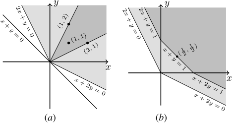
by Λ, i.e., the smallest convex cone containing Λ (this is the darkly shaded region in Figure 1(a)). Elements of co(Λ) are said to be positive linear combinations of elements of Λ.
Based on the principal idea in conventional SVM [Cortes and Vapnik, 1995], SVMRank picks a single w from the feasible set that maximises the margin (leading to a stronger ordering than ≽CΛ ); by margin we mean the perpendicular distance between the hyperplane Hw and the closest element of Λ to Hw. In simple terms, maximising the margin means choosing a feasible hyperplane that is as far as possible from Λ. This chosen hyperplane is equal to the hyperplane Hw where w uniquely has the minimum (Euclidean) norm in Λ≥ (see e.g., Theorem 1 in [Wilson and Montazery, 2016] for a proof). Let us denote this unique solution by ω∗Λ . In Figure 1(b), ( 1 2 , 1 2 ) has minimal norm in Λ≥, so ω∗Λ = ( 12 , 12 ), and thus, the associated hyperplane for that point, x+y = 0 in Figure 1(a), has the maximum margin. We use ‖w‖ as the notation for norm in this paper.
Definition 1 (≽mm Λ ). We define relation ≽mm Λ by, for α, β ∈ IRn , α is max-margin-preferred to β with respect to Λ (i.e., α ≽mm Λ β) if and only if α · ω∗Λ ≥ β · ω∗Λ , where ω∗Λ has minimum norm in Λ≥.
The relation ≽mm Λ is a total pre-order, since it is transitive and for any α, β ∈ IRn we have α ≽mm Λ β or β ≽mm Λ α (or both).
3 Rescaling of Preference Inputs
Consider the effect of rescaling the preference inputs Λ by t ∈ IR|Λ| + (where IR+ is the set of strictly positive reals), so that Λ becomes Λt = {t(i)λi : i ∈ I}, with each preference input being multiplied by a strictly positive scalar. We then have Λ≥t = {w ∈ IRn : ∀i ∈ I, w · (t(i)λi) ≥ 1}. We'll write t(i) as ti for brevity. Let us say that α is max-marginpreferred to β under rescaling t if α ≽mm Λt β. Now, it can easily happen that α is preferred to β under one rescaling, but not under another. To illustrate, consider t = (3, 1, 5) rescaling Λ in Example 1. Then, Λt will be {(6, 3), (1, 2), (5, 5)}, and it can be shown that the hyperplane with the maximum margin for Λt is x + 2y = 0 (instead of x + y = 0). Then, (2, -1.5) ≽mm Λ (0, 0), whereas (2,-1.5) ̸≽mm Λt (0, 0).
However, it seems natural to assume that if the user prefers ai over bi then he will also prefer tiai over tibi for any ti ∈ IR+. Also, for test vectors α and β, if α ≽mm Λ β then, for any positive real r, we have rα ≽mm Λ rβ; since the resultant preferences are invariant to such rescaling, it seems reasonable that the same would hold for the input preferences.
We therefore consider a more robust relation, which is invariant to the scaling of the preference inputs, with α being preferred to β only if it is preferred for all rescalings t ∈ IR|Λ| + of the preference inputs.
Definition 2 (≽IΛ). We define relation ≽IΛ by, for α, β ∈ IRn , α ≽IΛ β if and only if α is max-margin-preferred to β over all rescalings of preference inputs, i.e., if for all t ∈ IR|Λ| + , α ≽mm Λt β.
So far, we have assumed that each component ti of t can be any strictly positive scalar. However, in Proposition 1, we will show that if each ti is restricted to be in (0, 1], the result for ≽IΛ relation will not change. This is not surprising, since, e.g., doubling each component of t will not change the relation ≽mm Λt . This simplification will be helpful in the computation of the ≽IΛ relation.
Proposition 1. Consider any Λ ⊆ IRn and any α, β ∈ IRn . Then, α ≽IΛ β if and only if for all t ∈ (0, 1]|Λ| , α ≽mm Λt β.
Now, let us define SI(Λ) to be the set consisting solely of ω∗Λt for all scalings t ∈ (0, 1]|Λ| ; i.e., SI(Λ) = {ω∗Λt : t ∈ (0, 1]|Λ| }. Then, we have:
For example, it can be shown that SI(Λ) in Figure 1 is the intersection of the darkly shaded regions in sub-figures (a) and (b) (see Theorem 9 below).
3.1 Characterisation of SI(Λ)
Here, we mathematically characterise SI(Λ); this will lead to a computational method for the ≽IΛ relation. First, let us define for any Λ ⊆ IRn , the set Λ∗ to be {w ∈ IRn : ∀λ ∈ Λ, w · λ ≥ 0} (the union of the shaded regions in Figure 1(b)). Proposition 5 below implies that SI(Λ) ⊆ Λ≥ and every element u ∈ SI(Λ) has minimum norm in Λ∗ + {u} (= {w+u : w ∈ Λ∗ }). The proof uses the following three lemmas.
Lemma 2. Consider any Λ ⊆ IRn , and any t ∈ (0, 1]|Λ| . Then, for any u ∈ Λ≥t we have Λ∗ +{u} ⊆ Λ≥t .
Lemma 3. Consider any Λ ⊆ IRn , and any u ∈ Λ≥. Then, there exists t ∈ (0, 1]|Λ| such that Λ≥t = Λ∗ + {u}.
Lemma 4. Consider any Λ ⊆ IRn , and any t ∈ (0, 1]|Λ| . Then, Λ≥t ⊆ Λ≥.
Proposition 5. Consider any u ∈ IRn . Then, u ∈ SI(Λ) if and only if u ∈ Λ≥ and u has minimum norm in Λ∗ + {u}. Thus, in particular, SI(Λ) ⊆ Λ≥.
Proof: ⇒: u ∈ SI(Λ) means that there exists t ∈ (0, 1]|Λ| such that u ∈ Λ≥t and u has theminimumnorm inΛ≥t , which, since Λ≥t ⊆ Λ≥ by Lemma 4, implies that u ∈ Λ≥. Now, u also has the minimum norm in Λ∗ + {u} because firstly, Λ∗ +{u} ⊆ Λ≥t fromLemma 2, and secondly, u is clearly in Λ∗ + {u} since 0 ∈ Λ∗ .
⇐: Assume now that u ∈ Λ≥ and u has the minimum norm in Λ∗ + {u}. By Lemma 3, there exists t ∈ (0, 1]|Λ| such that u has the minimum norm in Λ≥t (= Λ∗ + {u}), and clearly u ∈ Λ≥t . Thus, u ∈ SI(Λ). ✷
We will prove (Proposition 8) that co(Λ) is precisely the set of elements u ∈ IRn such that u has minimum norm in Λ∗ + {u}. Together with Proposition 5, this will imply Theorem 9 below. The following two lemmas are used in the proof.
Lemma 6. Consider any u ∈ G where G ⊆ IRn is a convex set. Then, u has the minimum norm in G if and only if for all v ∈ G, u · (v - u) ≥ 0.
Lemma 7. Consider any Λ ⊆ IRn and any u ∈ IRn . Then, Λ∗ ⊆ {u}∗ if and only if u ∈ co(Λ).
Proposition 8. Consider any Λ ⊆ IRn and any u ∈ IRn . Then, u has minimum norm in Λ∗ + {u} if and only if u ∈ co(Λ).
Proof: Clearly, Λ∗ + {u} is a convex set. Lemma 6 implies that u has minimum norm in Λ∗ + {u} if and only if for all v ∈ Λ∗ +{u}, u· (v-u) ≥ 0. By writing y = v-u, this is if and only if for all y ∈ Λ∗ , u · y ≥ 0, which holds if and only if for any y ∈ Λ∗ , y ∈ {u}∗ . Thus, u has minimum norm in Λ∗ + {u} if and only if Λ∗ ⊆ {u}∗ . Lemma 7 then implies the result. ✷
Propositions 5 and 8 immediately imply the following theorem.
Theorem 9. Consider any Λ ⊆ IRn , any u ∈ IRn . Then, SI(Λ) = co(Λ) ∩ Λ≥.
This implies the following result, which leads immediately to an algorithm to determine, for arbitrary α, β ∈ IRn if α ≽IΛ β, using a linear programming solver.
Corollary 10. For finite set Λ ⊂ IRn , let λi ∈ Λ be the ith element of Λ where i ∈ I = {1, . . . , |Λ|}. Consider any u ∈ IRn . Then, u is in SI(Λ) if and only if there exist nonnegative reals ri for each i ∈ I such that u = ∑i∈I riλi and for all i ∈ I, u · λi ≥ 1.
4 Rescaling of Preference Inputs and Features
Scaling (normalization) of features is a necessary phase in any SVM-based method because these methods are not invariant to the rescaling of their input feature spaces [Stolcke et al., 2008; Ben-Hur and Weston, 2010]: multiplying a feature dimension by a fixed constant > 1 gives that dimension more weight in the choice of the feasible weight vector with minimum norm. This suggests defining another preference relation by considering the rescaling of features (so that each feature is rescaled by a strictly positive scalar across all preference inputs). This relation has been extensively analysed in [Wilson and Montazery, 2016] and is briefly described in Section 4.1. It is also natural to consider both kinds of rescaling simultaneously: preference inputs and features. In Section 4.2, we define and characterise a preference relation based on both kinds of rescaling.
4.1 Rescaling of Features
A features rescaling τ ∈ IRn+ is a vector of strictly positive numbers, with the jth component τ(j) being the scale factor for the jth feature. The effect of the rescaling on a vector u ∈ IRn is given by pointwise multiplication, u ⊙ τ , defined by for all j = 1, . . . , n, (u⊙τ)(j) = u(j)τ(j). The rescaling also changes the preference inputs Λ, turning it into Λ ⊙ τ, i.e., {λ⊙ τ : λ ∈ Λ}.
Definition 3 (≽FΛ). We define relation ≽FΛ by, for α, β ∈ IRn , α ≽FΛ β if and only if α is max-margin-preferred to β over all rescalings of features, i.e., if for all τ ∈ IRn+, we have α ⊙ τ ≽mm Λ⊙τ β ⊙ τ.
Proposition 11 below gives a representation of the relation ≽FΛ in terms of the set SF(Λ), consisting of all those elements in Λ≥ that have minimal rescaled norm for some feature rescaling.
Definition 4 (SF(Λ)). We define SF(Λ) by u ∈ SF(Λ) if and only if u ∈ Λ≥ and there exists some strictly positive τ ∈ IRn+ with ||τ ⊙ w|| ≥ ||τ ⊙ u|| for all w ∈ Λ≥.
Proposition 1 of [Wilson and Montazery, 2016] implies the following:
Proposition 11. For α, β ∈ IRn , α ≽FΛ β if and only if for all w ∈ SF(Λ), w · α ≥ w · β.
We say that u, v ∈ IRn agree on signs if, for each component j, u(j) and v(j) have equal sign: positive, negative or zero (this holds if and only if there exists some τ ∈ IRn+ with u ⊙ τ = v). Theorem 5 of [Wilson and Montazery, 2016] easily implies the following, which leads to a computational method for checking dominance with respect to ≽FΛ.
Theorem 12. Consider any Λ ⊆ IRn , any u ∈ IRn . Then, u is in SF(Λ) if and only if u ∈ Λ≥ and there exists µ ∈ IRn that agrees on signs with u such that µ ∈ co({λ ∈ Λ : λ · u = 1}). In particular, SF(Λ) ⊆ Λ≥.
4.2 Simultaneous Rescaling of Features and Inputs
We now consider a preference relation based on allowing both the rescaling of features and of preference inputs.
Definition 5 (SIF(Λ) and ≽I,F Λ ). We define the set SIF(Λ) by w ∈ SIF(Λ) if there exists t ∈ (0, 1]|Λ| such that w ∈ SF(Λt). We define relation ≽I,F Λ by α ≽I,F Λ β ⇐⇒ for all w ∈ SIF(Λ), w · α ≥ w · β.
This definition implies that α ≽I,F Λ β if and only if for all rescalings of the features and the preference inputs, α is maxmargin preferred to β. We have the following characterisation, which leads to a computational method for checking if α ≽I,F Λ β.
Theorem 13. u ∈ SIF(Λ) if and only if u ∈ Λ≥ and there exists µ ∈ IRn that agrees on signs with u such that µ ∈ co(Λ).
In Figure 1(b), SIF(Λ) is the part of the dark shaded region that is strictly within the first quadrant (so not including the axes), and SF(Λ) is the part of the line segment x + y = 1 strictly within the first quadrant.
5 Computation of Inferences
For finite subsets Λ of IRn , and arbitrary α, β ∈ IRn , we would like to be able to determine if α ≽CΛ β, α ≽IΛ β, α ≽FΛ β and α ≽I,F Λ β. Label Λ as {λi : i ∈ I}.
- ≽CΛ ≽CΛ ≽CΛ : α ̸≽CΛ β if and only if there exists u ∈ Λ≥ such that u · β > u · α. This holds if and only if there exists u ∈ IRn , such that u·(β-α) > 0 and ∀i ∈ I, u·λi ≥ 1.
≽IΛ ≽IΛ ≽IΛ: α ̸≽IΛ β if and only if there exists u ∈ SI(Λ) such that u · β > u · α. This holds, by Corollary 10, if and only if there exists u ∈ IRn , and non-negative reals ri for each i ∈ I, such that u · (β - α) > 0, ∀i ∈ I, u · λi ≥ 1; and u = ∑i∈I riλi.
- ≽FΛ ≽FΛ ≽FΛ: α ̸≽FΛ β if and only if there exists u ∈ SF(Λ) such that u · β > u · α. This holds, by Theorem 12, if and only if there exists u ∈ IRn and µ ∈ IRn , and non-negative reals ri for each i ∈ I, such that u · (β -α) > 0, and
- ∀i ∈ I, u · λi ≥ 1 and [u · λi = 1 or ri = 0];
- µ = ∑i∈I riλi;
- ∀j = 1, . . . , n, u(j) = 0 ⇐⇒ µ(j) = 0, and u(j) > 0 ⇐⇒ µ(j) > 0.
- ≽I,F Λ ≽I,F Λ ≽I,F Λ : α ̸≽I,F Λ β if and only if there exists u ∈ SIF(Λ) such that u·β > u·α. This holds, by Theorem 13, if and only if there exists u ∈ IRn and µ ∈ IRn , and non-negative reals ri for each i ∈ I, such that u · (β -α) > 0, and
- ∀i ∈ I, u · λi ≥ 1; µ = ∑i∈I riλi;
- ∀j = 1, . . . , n, u(j) = 0 ⇐⇒ µ(j) = 0, and u(j) > 0 ⇐⇒ µ(j) > 0.
These four relations, as well as ≽mm Λ , are all reflexive and transitive, and thus pre-orders (with ≽mm Λ being a total pre-order). We have that ω∗Λ ∈ SI(Λ) ∩ SF(Λ) and SI(Λ) ∪ SF(Λ) ⊆ SIF(Λ) ⊆ Λ≥. This implies that ≽mm Λ ⊇ ≽IΛ ∪ ≽FΛ, and ≽IΛ ∩ ≽FΛ⊇ ≽I,F Λ ⊇ ≽CΛ . Also, if ≽ is any of the five relations then λ ≽ 0 for any λ ∈ Λ; and for α, β, γ ∈ IRn and r ∈ IR+, if α ≽ β then α+γ ≽ β +γ and rα ≽ rβ.
6 Optimality Operators
In many decision making situations, there is no clear ordering on decisions (alternatives). There can often be a set of different scenarios with a different ordering on alternatives in each scenario. For example, for different scalings of preference inputs we may have different orderings over a set of alternatives. In such a setup there are a number of natural ways of defining the set of optimal solutions (best alternatives or top recommended solutions). We consider here two kinds of optimality operators; namely the set of undominated solutions, which is a natural generalisation of the Pareto-optimal set; and the set of possibly optimal solutions. The set of possibly optimal alternatives has been considered in a number of different situations, including for voting rules [Xia and Conitzer, 2008], for soft constraint optimisation [Rossi et al., 2011], and for multi-objective optimisation [Wilson et al., 2015b].
| |Λ| | Decisive Pairs (%) | Time (msec) | ||||||||
|---|---|---|---|---|---|---|---|---|---|---|
| ≽FΛ | ≽IΛ | ≽I∧F | ≽I,F Λ | ≽CΛ | ≽FΛ | ≽IΛ | ≽I,F Λ | ≽CΛ | ||
| 1. | 24 | 21 | 16 | 9 | 3 | 1 | 517 | 36 | 55 | 18 |
| 2. | 29 | 92 | 31 | 31 | 26 | 0.3 | 2434 | 23 | 40 | 16 |
| 3. | 31 | 23 | 28 | 13 | 1 | 0.1 | 800 | 25 | 38 | 13 |
| 4. | 36 | 81 | 35 | 35 | 31 | 23 | 4768 | 24 | 43 | 14 |
| 5. | 38 | 36 | 19 | 17 | 5 | 2 | 2799 | 24 | 47 | 17 |
| 6. | 41 | 61 | 12 | 12 | 12 | 12 | 5123 | 23 | 45 | 20 |
| 7. | 53 | 40 | 20 | 19 | 19 | 19 | 1134 | 24 | 41 | 20 |
| 8. | 55 | 97 | 26 | 26 | 24 | 8 | 1833 | 26 | 45 | 19 |
| 9. | 62 | 48 | 24 | 24 | 11 | 1 | 4983 | 27 | 50 | 14 |
| 10. | 94 | 64 | 35 | 35 | 5 | 2 | 5084 | 27 | 54 | 23 |
| 11. | 127 | 62 | 24 | 24 | 24 | 13 | 6439 | 28 | 57 | 21 |
| 12. | 129 | 80 | 36 | 36 | 19 | 1 | 2928 | 30 | 49 | 25 |
| 13. | 134 | 69 | 28 | 28 | 28 | 16 | 7374 | 30 | 48 | 19 |
| Avg. | 66 | 59 | 26 | 24 | 16 | 8 | 3555 | 27 | 48 | 19 |
Let ≽ be any of the relations ≽CΛ ,≽IΛ,≽FΛ and ≽I,F Λ , and let S be the corresponding set of scenarios for each relation (different scenarios means e.g., different scalings), which are respectively Λ≥, SI(Λ), SF(Λ) and SIF(Λ). We have then α ≽ β if and only if, for all u ∈ S, u · α ≥ u · β. We define ≻ to be the strict part of ≽, so that α ≻ β if and only if α ≽ β and β ̸≽ α.
For a given set of alternatives A, the two optimality operators are defined as follows:
- UNDS(A) (= UND≻(A)) is the set of undominated elements with respect to relation ≻, i.e., α ∈ UNDS(A) if and only if there is no β ∈ A such that β ≻ α.
- POS(A) is the set of elements that are optimal in some scenario. Thus, α ∈ POS(A) if and only if there exists u ∈ S such that for all β ∈ A, α · u ≥ β · u.
Typically (and as we found in our experiments), POS(A) is a smaller set than UNDS(A), although an alternative could be possibly optimal without being undominated.
Propositions 2 and 4 in [Wilson et al., 2015b] imply that the computation of both UNDS(A) and POS(A) can be done incrementally, and we exploit this for each of the relations ≽CΛ , ≽IΛ, ≽FΛ and ≽I,F Λ .
7 Experimental Testing
The experiments make use of a subset of a year's worth of real ridesharing records. These were provided by a commercial ridesharing system Carma (see http://gocarma.com/). We base our experiments on 13 benchmarks derived from this data set. Each ridesharing alternative has 7 features, representing different aspects of a possible choice of match for a given user. Each benchmark corresponds to the inferred preferences of a different user. The preference of alternative ai over bi leads to ai -bi(= λi)
| |POS(A)| | |UNDS(A)| | |||||||||
|---|---|---|---|---|---|---|---|---|---|---|
| C | I, F | I | F | I ∩F | C | I, F | I | F | I ∩F | |
| 1. | 38 | 26 | 20 | 6 | 4 | 72 | 55 | 33 | 16 | 13 |
| 2. | 45 | 13 | 12 | 2 | 2 | 86 | 20 | 15 | 3 | 3 |
| 3. | 64 | 37 | 21 | 6 | 5 | 97 | 74 | 30 | 19 | 18 |
| 4. | 7 | 7 | 7 | 3 | 3 | 7 | 7 | 7 | 4 | 4 |
| 5. | 33 | 32 | 21 | 13 | 12 | 63 | 54 | 38 | 17 | 17 |
| 6. | 14 | 14 | 14 | 5 | 5 | 18 | 18 | 18 | 5 | 5 |
| 7. | 10 | 10 | 10 | 6 | 6 | 18 | 18 | 17 | 7 | 7 |
| 8. | 18 | 9 | 9 | 1 | 1 | 25 | 12 | 12 | 1 | 1 |
| 9. | 34 | 17 | 13 | 6 | 6 | 78 | 19 | 15 | 8 | 8 |
| 10. | 22 | 15 | 8 | 2 | 2 | 50 | 38 | 13 | 2 | 2 |
| 11. | 20 | 14 | 14 | 2 | 2 | 27 | 19 | 19 | 3 | 3 |
| 12. | 41 | 12 | 9 | 2 | 2 | 79 | 24 | 15 | 2 | 2 |
| 13. | 16 | 12 | 12 | 4 | 4 | 29 | 16 | 16 | 6 | 6 |
| Avg. | 28 | 17 | 13 | 4 | 4 | 50 | 29 | 19 | 7 | 7 |
being included in Λ. However, a pre-processing phase deletes some elements of Λ, in order to make it consistent (i.e., Λ≥ ̸= ∅), since in this paper we assume consistent preferences. More information about the data can be found in [Montazery and Wilson, 2016]. To conduct the experiments, CPLEX 12.6.3 is used as the solver on a computer facilitated by an Intel Xeon E312xx 2.20 GHz processor and 8 GB RAM memory.
7.1 Decisive Pairs
Here, we would like to examine how decisive each relation is, i.e., which relation is weaker and by how much. We randomly generate 1000 pairs (α, β), based on a uniform distribution for each feature. A pair (α, β) is called decisive for a preference relation if one of them can (strictly) dominate the other one; for example, the pair (α, β) is decisive for ≽IΛ if and only if α ≻IΛ β or β ≻IΛ α. This is iff either (α ≽IΛ β and β ̸≽IΛ α) or (β ≽IΛ α and α ̸≽IΛ β). We also consider another relation ≽I∧F Λ which is the intersection of ≽IΛ and ≽FΛ, so that α ≽I∧F Λ β ⇐⇒ α ≽IΛ β and α ≽FΛ β.
Table 1 shows the percentage of decisive pairs for ≽FΛ, ≽IΛ, ≽I∧F Λ , ≽I,F Λ and ≽CΛ , as well as the running time per pair. Although for most of the benchmarks, ≽FΛ is more decisive than ≽IΛ, the third benchmark (bold numbers) shows that this is not always the case. In terms of running time, ≽IΛ is around 130 times faster than ≽FΛ on average. Also, the results illustrate the fact that ≽CΛ ⊆≽I,F Λ ⊆≽I∧F Λ .
7.2 Optimal Elements
The next phase of experiments is devoted to finding optimal solutions with respect to the two kinds of optimality operator discussed in Section 6. To do so, a set of 100 alternatives (i.e., the set A) is randomly generated, based on a uniform distribution for each feature. Then, for each relation, the number of possibly optimal and undominated elements in A is counted; see Table 2. The numbers in the I ∩ F columns relate to the intersection of the I and F optimality sets; for example, the left-hand I ∩F column gives the cardinalities of the sets POSI(Λ) ∩POSF(Λ). The bold numbers show that the F and I ∩ F columns are not identical, and thus illustrate that e.g., POSF(Λ) is not always a subset of POSI(Λ). It can be seen that for the most conservative relation, ≽CΛ , the optimality operators return a substantial proportion of alternatives as optimal solutions (roughly half for UNDS(A)).
| POS(A) Time (s) | UNDS(A) Time (s) | |||||||
|---|---|---|---|---|---|---|---|---|
| C | I, F | I | F | C | I, F | I | F | |
| 1. | 31 | 53 | 18 | 84 | 215 | 187 | 97 | 208 |
| 2. | 41 | 39 | 22 | 676 | 152 | 46 | 24 | 536 |
| 3. | 37 | 103 | 17 | 306 | 176 | 241 | 43 | 731 |
| 4. | 7 | 11 | 13 | 25 | 9 | 18 | 10 | 955 |
| 5. | 13 | 29 | 22 | 723 | 124 | 166 | 68 | 1491 |
| 6. | 17 | 22 | 21 | 353 | 32 | 53 | 29 | 1651 |
| 7. | 11 | 14 | 17 | 121 | 24 | 32 | 21 | 354 |
| 8. | 13 | 16 | 8 | 427 | 42 | 20 | 12 | 254 |
| 9. | 26 | 34 | 9 | 498 | 162 | 42 | 23 | 1549 |
| 10. | 27 | 31 | 14 | 855 | 151 | 136 | 25 | 1125 |
| 11. | 15 | 27 | 13 | 558 | 51 | 48 | 33 | 1759 |
| 12. | 41 | 23 | 14 | 482 | 272 | 46 | 22 | 585 |
| 13. | 27 | 24 | 19 | 724 | 68 | 46 | 29 | 2258 |
| Avg. | 24 | 33 | 16 | 449 | 114 | 83 | 34 | 1035 |
Table 3 shows the time for finding possibly optimal solutions and undominated solutions, where the former is faster than the latter by a factor ranging from 2.5 to 4.8 on average; this is partly because of |POS(A)| being usually much smaller than |UNDS(A)|, sometimes almost half the size, as shown in Table 2. Because the computation of ≽FΛ was very much slower than the other relations, the times in the F columns are much longer, despite the number of optimal solutions being smaller. Overall, the computational cost of the ≽FΛ may make it less useful, even though it is more decisive, and thus leads to smaller sets of optimal solutions. Instead one might, for instance, favour POSI(Λ), POSIF(Λ) and UNDSI(Λ) since they generate reasonably sized optimality sets much faster.
8 Summary and Discussion
In many situations, it can be argued that the scaling of preference inputs should not affect the induced preference relation. We have defined a relation ≽IΛ that is a more robust version of the maximum margin preference inference ≽mm Λ , and which is invariant to the scaling of preference inputs. This relation can be seen as complementary to the relation ≽FΛ [Wilson and Montazery, 2016], which is invariant to the way that features are scaled, leading to another preference relation ≽I,F Λ when both types of scalings are considered simultaneously. We derived characterisations for the new relations ≽IΛ and ≽I,F Λ , which lead to computational procedures. Our experiments, which used benchmarks derived from real preference data, compared the different relations, along with two different kinds of optimal alternative, and showed that the computational methods are practically feasible. The relation associated with only scaling the features was the most decisive but by far the slowest for computing the associated optimality classes.
In the future, it would be interesting to explore extensions of our approaches including (i) considering soft margin optimisation, i.e., dealing with the situation when preference inputs are inconsistent (e.g., one idea involves adding m extra real variables, one for each λ, in a way that ensures that the new feasible set is always non-empty); (ii) developing computational methods for certain kinds of kernel; and (iii) analysing the complexity of the computational methods.
Application for Imprecise Probability
Suppose we restrict the feasible w to being in the positive quadrant of IRn (this can be done by adding n unit vectors to Λ; or, perhaps better, by adding non-strict linear constraints enforcing non-negativity in an additional set Θ as defined in the formalism of [Wilson and Montazery, 2016]). Feasible w can then be viewed as unnormalised probability distributions on a sample space of n elements, and the input set Λ can be used to represent linear restrictions on probability distributions, or, as strictly acceptable gambles, in a theory of imprecise probability (or probabilistic logic) [Walley, 1991; 1996; Nilsson, 1986; Augustin et al., 2014]. Such linear restrictions, in particular, can represent upper and lower bounds on the conditional probabilities of propositions (subsets of the sample space).
Viewed in this light, the different approaches described in this paper generate different imprecise probability methods: upper and lower bounds on expectations of random variables, and of probabilities of propositions, can be computed using optimisation problems based on the models in Section 5. The cone-based relation ≽CΛ corresponds to standard upper and lower probability/prevision. A drawback of straight-forward upper and lower probability is that the consequent intervals of probability can sometimes be disappointingly weak. Our approaches give less conservative inference procedures (as implied by Theorems 9, 12 and 13, and backed up by our experimental results), whilst still satisfying natural invariance properties. The invariance to scaling of preference inputs is especially desirable in this context, since, for r > 0, the vector rλ represents the same restriction on probability distributions as λ; in terms of gambles, it corresponds to invariance to strictly positive scaling of the stakes. It would be very interesting, therefore, to explore the methods corresponding to ≽IΛ and ≽I,F Λ as approaches for reasoning with imprecise probability.
Acknowledgments
This publication has emanated from research conducted with the financial support of Science Foundation Ireland (SFI) under Grant Number SFI/12/RC/2289. Thanks to the reviewers for their comments, which helped improve the final version of the paper.
@inproceedings{ijcai2017p168,
  title     = {Dominance and Optimisation Based on Scale-Invariant Maximum Margin Preference Learning},
  author    = {Montazery, Mojtaba and Wilson, Nic},
  booktitle = {Proceedings of the Twenty-Sixth International Joint Conference on
               Artificial Intelligence, {IJCAI-17}},
  publisher = {International Joint Conferences on Artificial Intelligence Organization},
  editor    = {Carles Sierra},
  pages     = {1209--1215},
  year      = {2017},
  month     = {8},
  note      = {Main track},
  doi       = {10.24963/ijcai.2017/168},
  url       = {https://doi.org/10.24963/ijcai.2017/168},
}
TY - CPAPER TI - Dominance and Optimisation Based on Scale-Invariant Maximum Margin Preference Learning AU - Montazery, Mojtaba AU - Wilson, Nic T2 - Proceedings of the Twenty-Sixth International Joint Conference on Artificial Intelligence, IJCAI-17 PB - International Joint Conferences on Artificial Intelligence Organization PY - 2017 SP - 1209 EP - 1215 DO - 10.24963/ijcai.2017/168 UR - https://doi.org/10.24963/ijcai.2017/168 ER -Copied
Machine-readable versions of this paper, for tools and AI agents:





