
Object-Based World Modeling in Semi-Static Environments with Dependent Dirichlet Process Mixtures
Proceedings of the Twenty-Fifth International Joint Conference on Artificial Intelligence. Pages 3513-3520.
© 2016 International Joint Conferences on Artificial Intelligence
Abstract
To accomplish tasks in human-centric indoor environments, agents need to represent and understand the world in terms of objects and their attributes. We consider how to acquire such a world model via noisy perception and maintain it over time, as objects are added, changed, and removed in the world. Previous work framed this as multiple-target tracking problem, where objects are potentially in motion at all times. Although this approach is general, it is computationally expensive. We argue that such generality is not needed in typical world modeling tasks, where objects only change state occasionally. More efficient approaches are enabled by restricting ourselves to such semi-static environments. We consider a previously-proposed clustering-based world modeling approach that assumed static environments, and extend it to semi-static domains by applying a dependent Dirichlet process (DDP) mixture model. We derive a novel MAP inference algorithm under this model, subject to data association constraints. We demonstrate our approach improves computational performance for world modeling in semi-static environments.
- [Ahmed and Xing, 2008] A. Ahmed and E. Xing. Dynamic non-parametric mixture models and the recurrent Chinese restaurant process: with applications to evolutionary clus- tering. In SIAM International Conference on Data Mining, 2008.
- [Antoniak, 1974] C.E. Antoniak. Mixtures of Dirichlet pro- cesses with applications to Bayesian nonparametric prob- lems. The Annals of Statistics, 2(6):1152-1174, 1974.
- [Bar-Shalom and Fortmann, 1988] Y. Bar-Shalom and T.E. Fortmann. Tracking and Data Association. Academic Press, 1988.
- [Besag, 1986] J. Besag. On the statistical analysis of dirty pictures. Journal of the Royal Statistical Society, Series B, 48:259-302, 1986.
- [Blei and Jordan, 2006] D.M. Blei and M.I. Jordan. Varia- tional inference for Dirichlet process mixtures. Bayesian Analysis, 1(1):121-143, 2006.
- [Cox and Leonard, 1994] I.J. Cox and J.J. Leonard. Model- ing a dynamic environment using a Bayesian multiple hy- pothesis approach. Artificial Intelligence, 66(2):311-344, 1994.
- [Dellaert et al., 2003] F. Dellaert, S.M. Seitz, C.E. Thorpe, and S. Thrun. EM, MCMC, and chain flipping for struc- ture from motion with unknown correspondence. Machine Learning, 50(1-2):45-71, 2003.
- [Elfring et al., 2013] J. Elfring, S. van den Dries, M.J.G. van de Molengraft, and M. Steinbuch. Semantic world modeling using probabilistic multiple hypothesis anchor- ing. Robotics and Autonomous Systems, 61(2):95-105, 2013.
- [Escobar and West, 1995] M.D. Escobar and M. West. Bayesian density estimation and inference using mix- tures. Journal of the American Statistical Association, 90(430):577-588, 1995.
- [Huang et al., 2015] R. Huang, F. Zhu, and P.-A. Heng. The dynamic Chinese restaurant process via birth and death processes. In AAAI Conference on Artificial Intelligence, 2015.
- [Jain and Neal, 2004] S. Jain and R.M. Neal. A split-merge Markov chain Monte Carlo procedure for the Dirichlet process mixture model. Journal of Computational and Graphical Statistics, 13(1):158-182, 2004.
- [Karp, 1972] R.M. Karp. Reducibility among combinato- rial problems. In R.E. Miller, J.W. Thatcher, and J.D. Bohlinger, editors, Complexity of Computer Computa- tions, pages 85-103. Springer US, 1972.
- [Kuhn, 1955] H.W. Kuhn. The Hungarian method for the assignment problem. Naval Research Logistics Quarterly, 2(1-2):83-97, 1955.
- [Lin et al., 2010] D. Lin, E. Grimson, and J. Fisher. Con- struction of dependent Dirichlet processes based on Pois- son processes. In Advances in Neural Information Pro- cessing Systems, 2010.
- [Lin, 2012] D. Lin. Generative Modeling of Dynamic Visual Scenes. PhD thesis, Massachusetts Institute of Technol- ogy, 2012.
- [Luo et al., 2015] W. Luo, B. Stenger, X. Zhao, and T.-K. Kim. Automatic topic discovery for multi-object tracking. In AAAI Conference on Artificial Intelligence, 2015.
- [MacEachern, 1999] S.N. MacEachern. Dependent nonpara- metric processes. In ASA Section on Bayesian Statistics, 1999.
- [MacEachern, 2000] S.N. MacEachern. Dependent Dirichlet processes. Technical report, Ohio State University, 2000.
- [Munkres, 1957] J. Munkres. Algorithms for the assignment and transportation problems. Journal of the Society for Industrial and Applied Mathematics, 5(1):32-38, 1957.
- [Murty, 1968] K.G. Murty. An algorithm for ranking all the assignments in order of increasing cost. Operations Re- search, 16(3):682-687, 1968.
- [Neal, 2000] R.M. Neal. Markov chain sampling methods for Dirichlet process mixture models. Journal of Compu- tational and Graphical Statistics, 9(2):249-265, 2000.
- [Neiswanger et al., 2014] W. Neiswanger, F. Wood, and E.P. Xing. The dependent Dirichlet process mixture of objects for detection-free tracking and object modeling. In Inter- national Conference on Artificial Intelligence and Statis- tics, 2014.
- [Oh et al., 2009] S. Oh, S. Russell, and S. Sastry. Markov chain Monte Carlo data association for multi-target track- ing. IEEE Transactions on Automatic Control, 54(3):481- 497, 2009.
- [Pasula et al., 1999] H. Pasula, S. Russell, M. Ostland, and Y. Ritov. Tracking many objects with many sensors. In International Joint Conference on Artificial Intelligence, 1999. IJCAI
- [Rauch et al., 1965] H.E. Rauch, F. Tung, and C.T. Striebel. Maximum likelihood estimates of linear dynamic systems. AIAA Journal, 3(8):1445-1450, 1965.
- [Reid, 1979] D.B. Reid. An algorithm for tracking mul- tiple targets. IEEE Transactions on Automatic Control, 24(6):843-854, 1979.
- [Teh, 2010] Y.W. Teh. Dirichlet processes. In C. Sammut and G.I. Webb, editors, Encyclopedia of Machine Learn- ing, pages 280-287. Springer US, 2010.
- [Wong et al., 2015] L.L.S. Wong, L.P. Kaelbling, and T. Lozano-Pérez. Data association for semantic world modeling from partial views. The International Journal of Robotics Research, 34(7):1064-1082, 2015.
- [Wong et al., 2016] L.L.S. Wong, T. Kurutach, L.P. Kael- bling, and T. Lozano-Pérez. Object-based world model- ing in semi-static environments with dependent Dirichlet- process mixtures. arXiv:1512.00573 [cs.AI], 2016.
- [Zhu et al., 2005] X. Zhu, Z. Ghahramani, and J. Lafferty. Time-sensitive Dirichlet process mixture models. Techni- cal report, Carnegie Mellon University, 2005.
References were extracted automatically from the PDF and may contain errors.
Full text extracted automatically from the PDF; figures, tables and equations may differ. The PDF is the version of record.
1 Introduction
Robots need to know about objects in order to perform most tasks in human-centered environments. Objects should be understood in terms of semantic attributes such as type, pose, function, and possibly relations with other objects. Semantic perception tools are increasingly becoming available, and it is tempting to use them as black-box perception modules. However, such perception is still error-prone, due to noise, occlusion, clutter, and limited fields of view. To achieve greater reliability, our strategy is to aggregate the output from noisy perception pipelines, across time and space (different viewpoints), and estimate the true state, i.e., the world model.
Estimating properties of individuals from noisy observations is a relatively simple statistical estimation problem if the observations are labeled according to which individual generated them. Even when the underlying attributes of the individual change over time, estimating their history reduces to inference in a hidden Markov model.
Thanard Kurutach, Tom´as Lozano-P´erez, Leslie Pack Kaelbling
MIT Computer Science and Artificial Intelligence Laboratory
Cambridge, MA 02139, USA
¶kurutach, tlp, lpk♦@csail.mit.edu
The key difficulty is data association. We do not know which particular individual is responsible for each observation; determining an appropriate association of observations to individuals is key. The only information we have to make such associations are noisy and partial observations, which may contain errors both in attribute values and in number.
This problem was first addressed in the context of multipletarget tracking [Bar-Shalom and Fortmann, 1988]. A classical solution is multiple hypothesis tracking [Reid, 1979], which has been applied in previous world modeling applications [Cox and Leonard, 1994; Elfring et al., 2013]. Oh et al. [2009] have pointed out drawbacks in using the MHT, which include inefficiency due to considering an exponential number of hypotheses, and the inability to revisit associations from previously-considered views (the MHT is a filtering algorithm). Inspired by this, they and others [Dellaert et al., 2003; Pasula et al., 1999] have proposed different Markovchain Monte Carlo (MCMC) methods for data association, and have demonstrated superior tracking performance.
In multiple-target tracking problems, each target's state (typically location) changes between observations. However, if we consider applications such as tracking objects in a household, the dynamics are different: most objects tend to stay in the same state when they are not being actively used. In this paper, we study the world modeling problem in semistatic environments, where time is divided into known epochs, and within each epoch the world is stationary. Intuitively, data association should be easier within static periods, since there is no uncertainty arising from stochastic dynamics.
At the other end of the spectrum, in previous work we considered the world modeling problem under a static world assumption [Wong et al., 2015]. We proposed a clusteringbased view of the problem, where objects are treated as cluster components (in a joint attribute space), and observations are noisy measurements generated from these clusters. We used Bayesian nonparametric models to handle an unknown number of objects, in particular the Dirichlet process mixture model (DPMM). This approach is fundamentally limited by the DPMM's inability to capture temporal dynamics.
Dependent Dirichlet processes (DDP), in contrast, are capable of modeling dynamic clusters. We use a DDP mixture model to infer object attributes and their changes over time, including the addition and removal of objects in the world. A novel approximate MAP inference method is also proposed.
2 ProblemDefinition
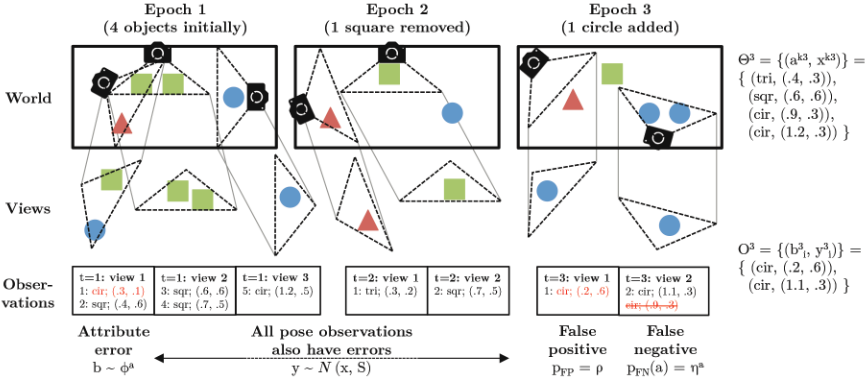
In world modeling, we seek the state of the world, consisting an unknown finite number Kt of objects, which changes over time. Object k at epoch t has attribute values ✓kt . We sometimes decompose ✓kt into (ak ↪ xkt ), where a is a vector of fixed attributes, and x is a vector of attributes that may change between epochs. The top row in Figure 1 illustrates the world state over three epochs for a simple domain.
Our system obtains noisy, partial views of the world. Each view v produces a set of observations Otv = ¶otv i ♦, where otv i = (btv i ↪ ytv i ), corresponding to the fixed attributes a and dynamic attributes xt of some (possibly non-existent) object. 1 Each view is also associated with a field of view V tv . The collection of views in a single epoch may fail to cover the entire world. The partial views and noisy observations are illustrated in the middle and bottom rows of Figure 1.
The world modeling problem can now be defined: Given observations O = ¶otv i ♦(t↪v↪i) and fields of view ¶V tv ♦(t↪v) , determine the state of objects over time ⇥ = {✓kt (k↪t) . The state includes not only objects' attribute values, but also the total number of objects that existed at each epoch, and implicitly when objects were added and removed (if at all).
There is no definitive information in the observations that will allow us to know which particular observations correspond with which underlying objects in the world, or even how many objects were in existence at any time step. For example, in the views of t = 1 shown in Figure 1, the square detected in the left-most view may correspond to either (or neither) square in the center view. Also, despite there being only four objects in the world, there were five observations because of overlapping visible regions.
1 Superscripts in variables will generally refer to the 'context', such as object index k and time index t. Subscripts refer to the index in a list, such as oti = i'th observation at time t.
The critical piece of information that is missing is the association ztv i of an observation otv i to an underlying object k. With this information, we can perform statistical aggregation of the observations assigned to the same object to recover its state. We will model the associations Z = ¶ztv i ♦(t↪v↪i) as latent variables in a Bayesian inference process.
2.1 Observation noise model
The observation model describes how likely an observation o = (b↪ y) was generated from some given object state ✓ = (a↪ x) (if any), given by the probability f (o ; ✓). For a single object, let ✓c and ✓d be the true continuous and discrete attribute values respectively, and likewise oc and od for a single observation of the object. We typically consider observation noise models of the following form:
Here φ represents a discrete confusion matrix, where φ✓d (od) is the probability of observing od given the true object has discrete attributes ✓d. The continuous-valued observation oc is the true value ✓c corrupted with zero-mean Gaussian noise, with fixed sensing covariance S. The noise on oc and od are assumed to be independent for simplicity.
2.2 Additional data association assumptions
Besides errors in attribute values, Figure 1 also illustrates cases of false positives and false negatives. A false positive occurs when the observation did not originate from any true object. We assume that this occurs at a fixed rate ⇢. When this occurs, od has noise distribution φ0 , and oc is uniformly distributed over the field of view V . A false negative occurs when an object is within the sensor's field of view but failed to be detected. We assume that an object within the field of view V will be undetected with probability ⌘(✓).
There is an additional common domain assumption in target-tracking problems: within a single view, each visible object can generate at most one detection [Bar-Shalom and Fortmann, 1988]. This implies that within a view, each observation must be assigned to a different hypothesized underlying object. In the parlance of clustering, we refer to this as the "cannot-link constraint" (CLC). The constraint is powerful because it can reduce ambiguities when there are similar nearby objects. However, we will need to modify the DDPMMmodel and inference algorithms to handle the CLC.
3 AClustering-Based Approach
We now specify a prior on how likely an assignment to a cluster is, and how clusters change over time. Since the number of clusters are unknown, we chose to use Bayesian nonparametric mixture models, which allow for an indefinite and unbounded number of mixture components.
The Dirichlet process (DP) (Teh [2010] provides a good overview) is a widely-studied prior for density estimation and clustering [Antoniak, 1974; Escobar and West, 1995; Neal, 2000]. The DP's popularity stems from its simplicity and elegance, and in previous work we have applied them to a similar (static) world modeling problem [Wong et al., 2015]. However, one major limitation is that clusters cannot change over time, a consequence of the fact that observations are assumed to be fully exchangeable. This assumption is violated for problems like ours, where the observed entities change over time. Various generalizations of the DP that model temporal dynamics have thus been proposed [Zhu et al., 2005; Ahmed and Xing, 2008; Neiswanger et al., 2014; Luo et al., 2015; Huang et al., 2015].
Many of these generalizations belong to a broad class of stochastic models known as dependent Dirichlet processes (DDP) [MacEachern, 1999; 2000]. We will adopt a theoretically-appealing instance of the DDP, based on a Poisson-process construction [Lin et al., 2010]. This construction subsumes a number of existing algorithmicallymotivated DP generalizations. Additionally, it has the nice property that at each time slice, the prior over clusters is marginally a DP. Given a DP prior at time t, the construction specifies a dependent prior at time t + 1 (or another future time), which is shown to also be a DP. The construction therefore generates a Markov chain of DPs over time, which reflects temporal dynamics between epochs in our problem.
We now restate one result of the DDP construction; see Lin [2012] for details. The construction results in the following prior on parameter ✓t (to be assigned to a new observation), given past parameters ⇥<t and parameters ⇥t for clusters that have already been instantiated at the current epoch:
At the initial time step, clusters are formed as in a standard DPMM with concentration parameter ↵ and base distribution H. For later time steps, the prior distribution on ✓ is defined recursively. The first two terms are similar to the base case, for new clusters and already-instantiated clusters (in the current epoch) respectively. The third term corresponds to previously-existing clusters that may be removed with probability (1-q(✓k↪t-1 )), and, if it survives, is moved with transition probability T (· ; ✓k↪t-1 ). N k↪t is the number of points that have been assigned to cluster k, for all time steps up to time t. If q ⌘ 1 and T (· ; ✓) = δ✓, then the model is static, and Equation 2 is equivalent to the DP predictive distribution.
3.1 Inference by forward sampling
As mentioned in the problem definition, our focus will be on determining latent assignments Z = ¶zt i ♦ of observations O = ¶oti ♦ to clusters with parameters ⇥ = {✓kt . In the generic DDP, views do not exist yet; those will be introduced in Section 4. One way to explore the distribution of assignments is to sample repeatedly from the assignment's conditional distribution, given all other assignments Z∩ti , Z ∩ ¶zt i ♦, found using Bayes' rule:
The first term in the integrand is given by the observation noise model (Equation 1), and the second term is given by the DDP prior (Equation 2). If ✓kt already exists, then P (✓ ∣∣ ⇥↪ Z∩ti ) = I ⇥✓ = ✓kt ⇤, and the integrand only has support for ✓ = ✓kt . Otherwise, we have to consider all possible settings of ✓kt , which has a prior distribution given by Equation 2. The expression in Equation 4 above can be decomposed into three cases, corresponding to terms in Equation 2:
In the DDPMM, clusters move around the parameter space during their lifetimes, and, depending on our chosen viewpoints, may not generate observations at some epochs. When cluster k has at least one time-t observation assigned to it, it becomes instantiated at time t. Any subsequent observations at time t that are assigned to cluster k must then share the same parameter ✓kt ; this corresponds to the first case. The second case is for clusters not yet instantiated at time t, and we must infer ✓kt from the last known parameter for cluster k, at time ⌧ < t. If t - ⌧ > 1, we use generalized survival and transition expressions for our application:
The third case is for new clusters that are added at time t.
In general, since the cluster parameters ⇥ are also unknown, they need to be sampled from their conditional distributions given Z. With additional assumptions presented next, we can find the parameter posterior distribution efficiently and avoid sampling the parameter entirely by 'collapsing' it.
3.2 Application of DDPs to world modeling
We now apply the DDP mixture model (DDPMM) to the semi-static world modeling problem. For simplicity, we consider an instance of the world modeling problem where the fixed attribute a is the discrete object type (from a finite list of known types), and the dynamic attribute x is the continuous pose in Rd (either 3-D location or 6-D pose). Despite these restrictions, our model and derivations can be immediately applied to problems with any fixed attributes, and with any dynamic continuous attributes with linear-Gaussian dynamics. Arbitrary dynamic attributes can be represented in our model, but inference will likely be more challenging because in general we will not obtain closed-form expressions. For our instance of the DDPMM, we assume:
- ÷ Time steps in the DDP correspond to epochs in world modeling, i.e., each epoch is modeled as a static DPMM.
- ÷ The survival rate only depends on the fixed attribute, i.e., q(✓) = q(a). (For us, that means the likelihood of object removal is dependent on the object type but not its pose.)
- ÷ Likewise, the detection probability only depends on the fixed attribute (object type), i.e., ⌘(✓) = ⌘(a).
- ÷ The dynamic attribute (pose) follows a random walk with zero-mean Gaussian noise that depends on a (e.g., a mug likely travels farther per epoch than a table):
This implies that the full transition distribution is (of both object type and pose) is:
- ÷ The DP base distribution has the following form:
We place a (discrete) prior ⇡ over the object type, and a noninformative normal distribution over the object pose, to allow for an object being introduced at any location.
The above choices for the dynamics and base distribution implies that the parameter posterior and predictive distributions have closed-form expressions. The posterior distribution of the dynamic attribute is a mixture of Gaussians, with a component for each possible value of the fixed attribute a (since the process noise R(a) may be different), weighted by the posterior probability of a. In practice, we track the pose using only the dynamics of the most-likely object type ˆak . Thus, in our application, each cluster maintains a discrete posterior distribution '(a) for the object type, and a Kalman filter or Rauch-Tung-Striebel (RTS) smoother [Rauch et al., 1965] for the object pose distribution. The latter is represented as a sequence of means and covariances ¶θkt ↪ ⌃kt ♦⇣t=⇠ over the cluster k's lifetime t 2 [⇠↪ ⇣], with the interpretation that xkt ⇠ N(θkt ↪⌃kt ). For more details and derivation of the parameter distributions, please refer to the extended version of our paper [Wong et al., 2016].
Because we have compact representations of the parameter posterior distributions, we can analytically integrate ⇥ out instead of sampling them. We first modify the forward sampling equation (Equation 5) to reflect this 'collapsing' operation. Since we can no longer condition on the parameters themselves, we instead need to condition on the other observations O∩ti and their current cluster assignments Z∩ti, and
use posterior predictive likelihoods of the form P ⇣oti ∣∣∣Ok ∩ti⌘ to evaluate the current observation oti :
We can now substitute the expressions for P (oti ∣∣ ✓kt ), ˜ T, and H, where properties of the normal distribution will help us evaluate the integrals. The derivations in Wong et al. [2016] give the following expressions, as well as details for finding the posterior hyperparameters ', θkt , and ⌃kt (recall that ✓kt = (ak ↪ xkt ) ↪ oti = (bti ↪ yt i )):
4 IncorporatingWorldModeling Constraints
So far, we have only applied a generic DDPMM to our observations, but have ignored false positives (FP), false negatives
(FN), and the cannot-link constraint (CLC). To capture these additional domain characteristics, we modify the conditional distribution from which samples are iteratively taken from:
The second product is the likelihood for all FP observations (ztv i = 0), which is basically the same as the new-cluster case in Equation 11, except for the N 0 ∩tv factor at the end. The similarity is intentional, since, given a single observation, an FP is indistinguishable from a new cluster. N 0 ∩tv is the number of other FPs observed, or, if none exist, then ↵ is used instead (to prevent the product being zero).
In the above, the correspondence vector ztv is the concatenation of the individual ztv i assignment variables, for all observation indices i made in view v at epoch t; the interpretation of otv is similar. The individual terms in the first product are given by Equation 11 (the value of ztv i determines which case applies). The product is over all observations that are not FPs (ztv i 6= 0), hence the (1-⇢) Bernoulli term.
The third product, for FNs, is a product over all clusters alive at time t. Recall that an object that is within the field of view fails to be detected with type-dependent probability ⌘(ak ). Let δtv k be 1 if cluster k is detected in viewv at epoch t, and 0 otherwise. For a cluster k that is alive at epoch t (⇠ k t ⇣ k ) with parameter ✓kt , the probability of detection is the probability it is within the field of view, and is not missed:
The ˜Φ function denotes the CDF of the multivariate normal distribution, with mean θkt and covariance ⌃kt . The detection indicator variables δtv k are determined during sampling by the correspondence vector ztv : if some element of otv is assigned to cluster index k, then δtv k = 1; otherwise, δtv k = 0.
Finally, the cannot-link constraint, described in Section 2.2, couples together cluster assignments for observations within the same view, since we must ensure that no two observations can be assigned to the same existing cluster. The final term in Equation 12 enforces this constraint. Invalid correspondence vectors that violate the cannot-link constraint are assigned zero probability and hence are not considered; the remaining conditional probabilities are normalized. This can be interpreted as performing blocked Gibbs sampling, where blocks are determined by the joint constraints.
Putting everything together, we arrive at a constrained blocked collapsed Gibbs sampling inference algorithm. The algorithm takes the observations O = ¶otv i ♦ and visible regions ¶V tv ♦ as input. As output, the algorithm produces samples from the posterior distribution over correspondence vectors ¶ztv ♦, from which we can compute the posterior parameter distributions ak ⇠ ' and xkt ⇠ N (θkt ↪ ⌃kt ). The sampling algorithm repeatedly iterates over epochs t and views v, each time sampling a new correspondence vector ztv from its constrained conditional distribution, given by Equation 12.
5 Approximate MAP Inference
We have now presented the entire Gibbs sampling algorithm for DDPMM-based world modeling. which generates samples from the posterior distribution of object states ⇥ (and object-observation assignments Z). However, samplingbased inference can be slow, especially because of the cannotlink constraint that couples together many latent variables. Although we are interested in maintaining an estimate of our uncertainty in the world, frequently just having the mostlikely (maximum a posteriori - MAP) world model suffices. In general, even the MAP is hard to find, because it can be formulated as a multidimensional assignment problem, which is known to be NP-complete for T ≥ 3 epochs [Karp, 1972]. Nevertheless, since it is a fundamental combinatorial problem, many approximate solutions have been proposed.
5.1 Iterated conditional modes (ICM)
The iterated conditional modes (ICM) algorithm performs coordinate ascent on each variable's conditional distribution, and is guaranteed to converge to a local maximum [Besag, 1986]. Instead of iteratively sampling correspondence vectors from their conditional distributions in Gibbs sampling, we find the most-likely one, update parameters based on it, and repeat for each view and epoch. The space of joint correspondence vectors is combinatorial in size, so finding the maximizer is still potentially inefficient. Fortunately, finding the most-likely correspondence for a single view can be formulated as a maximum weighted assignment problem, for which cubic-time exact algorithms such as the Hungarian algorithm exist (and have been used in data association) [Kuhn, 1955; Munkres, 1957; Murty, 1968].
Suppose, for view v at epoch t, there are M observations ¶o1↪ ▷ ▷ ▷ ↪ oM♦ and K existing clusters (possibly not alive/instantiated). Then we wish to match each oi to an existing cluster, a new cluster, or a false positive. Any unmatched existing cluster must also be assigned the probability of missed detection. We can solve this as an assignment problem with the following payoff matrix:
| Obs (M cols) | FN (M + K) | |
|---|---|---|
| Clusters (K rows) | log P (zi = k) + log(1 - ⇢) +I ⇥⇠k t ⇣ k ⇤ logP(δk = 1) | I ⇥⇠k t ⇣ k ⇤ logP(δk = 0) |
| New (M) | logP(zi = new) + log(1-⇢) | 0 |
| FP (M) | log P (zi = 0 (FP)) + log ⇢ | 0 |
The payoff matrix has 2M + K entries to allow for the case that all observations are assigned to new clusters, and likewise that all are spurious. Any extra New/FP nodes are assigned to extra FN nodes, with zero payoff. The payoffs in
Input: Obs. O = {otv i , Visible regions {V tv , Num. samples N Output: Samples of cluster assignments {ztv
- 3: for t := 1 to T ; v := 1 to V t do
- 1: Init. all entries to -1 (FP) in Z (0) = {ztv (0) 2: repeat
- 4: Solve assignment problem for most-likely ztv , given Z t∩v
- 5: until convergence
- 7: Sample tracks by performing MCMCDA on C
- 6: Construct a new dataset C = {cti with a single data point for each non-FP cluster found by ICM (above) at each epoch
- 8: Convert track samples to cluster assignments
Figure 2: ICM-MCMC, a two-stage inference algorithm for DDPMM, using ICM and MCMCDA [Oh et al., 2009].
the first column are: for an existing cluster, given by cases 1 and 2 in Equation 11, depending on whether or not the cluster has been instantiated yet; for a new cluster, given by case 3 in Equation 11; and for an FP, given within the second product of Equation 12. Log probabilities decompose the view's joint correspondence probability into a sum of individual terms. By construction, the cannot-link constraint is satisfied. Since all terms in Equation 12 are exactly accounted for in the constructed payoff matrix, the maximum assignment found through this procedure yields the joint correspondence vector that maximizes the conditional distribution (Equation 12), given all other associations. Iterating this procedure for each view and epoch thus yields an ICM algorithm and produces an approximate MAP solution.
5.2 A two-stage inference scheme
Although the ICM algorithm presented can find good clusters at a single epoch very quickly, we will see in experiments that it does not converge to good cluster trajectories. The issue is that ICMmoves are local, in that it considers one view at a time. Suppose we have identified correctly all objects in epoch 1 using ICM. When we consider the first view in epoch 2, there may be significant changes present, and using observations from the first view only, ICM must decide whether or not to assign the new observations to existing clusters (by reviving them). Since the uncertainty in the object states immediately after a transition is high, basing the cluster connectivity decisions on a single view is unreliable.
This suggests a two-level inference scheme. Since ICM can reliably find good clusters within single epochs, we first apply ICM to each epoch's data independently, treating them as unrelated static worlds. Next, we attempt to connect clusters between different epochs. This is essentially another tracking problem, although the likelihood function is somewhat different (depends on many underlying data points), and is much reduced in size. Since the problem is significantly smaller, tracking methods such as MHT or MCMCDA can be applied to this cluster-level tracking problem.
We present one such scheme in Algorithm 2, using MCMCDA [Oh et al., 2009] to solve the cluster-level problem. We choose a batch-mode sampling algorithm such as MCMCDA because it can return samples from the posterior distribution, and has an attractive anytime property - we can terminate at any point and still return a list of valid samples. For inferring the MAP configuration, the best sample can be returned instead. Since we are sampling from the true posterior distribution (assuming that the per-epoch clusters are identified correctly), in the limit of infinite samples, the true MAP configuration will be found almost surely.
6 Experiments
Approximate MAP inference for world modeling via ICM, MCMCDA, and the two-stage ICM-MCMC were tested on a simulated domain, and on a sequence of robot vision data constructed from the static scenes in Wong et al. [2015]. To perform MAP inference on MCMCDA and ICM-MCMC, the most-likely sample was chosen, from 105 samples in MCMCDA, and 104 in the second stage of ICM-MCMC. We find that ICM-MCMC significantly outperforms the other two methods, and even ICM performs better than MCMCDA.
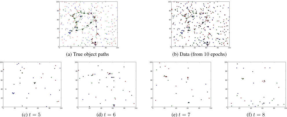
We used a simulated domain similar to the one given in the MCMCDA paper [Oh et al., 2009]. Objects in our version had one of four fixed object types, a time-evolving location (x↪ y) 2 [0↪ 100] ⇥ [0↪ 100], and a time-evolving velocity vector. Observations were made in 10 epochs of this domain, with 5 views per epoch (visible region is the entire domain). In total, 5 objects existed, each for some contiguous sub-interval of the elapsed time. Noise parameters were similar to Oh et al. [2009]. The observed data and the true object states from one trial (of 100) are shown in Figure 3.
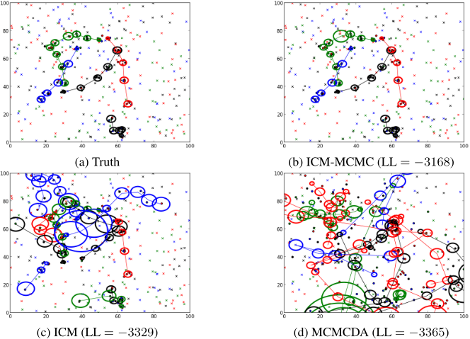
The resulting MAP clusters found by ICM, MCMCDA, and ICM-MCMC for a representative trial are shown in Figure 4, along with their log-likelihood values (higher / less negative is better). ICM-MCMC clearly outperforms the other methods, and finds essentially the same clusters as given by the true association. The clusters found generally have tight covariance values, unlike those in ICM and MCMCDA. These two methods, especially MCMCDA, tend to find many more clusters than are truly present. Due to the large number of candidates (neighbors) in MCMCDA, it fails to one that explains all the data. In contrast, by running ICM first, and performing MCMCDA on the found clusters, the search space is greatly reduced and the algorithm performs well.
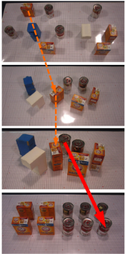
We also applied the same algorithms to the static robot vision data from Wong et al. [2015]. To convert static scenes into dynamic scenes, we choose static scenes that were reasonably similar, and simply concatenated their data together, as if each scene corresponded to a different epoch. One such example is shown in Figure 5. Objects in different scenes were all placed on the same tabletop. Four object types were present, and typically each scene had 5-10 objects. Object types and poses were detected using a black-box object detector; see Wong et al. [2015] for details about the data and noise models. Unlike the simulation, objects do not have velocities. Instead, between epochs, we assume that the location changes with isotropic Gaussian noise, standard deviation 0▷1. Since changes were significant between epochs, we assumed a relatively low 0▷5 probability of survival.
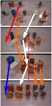
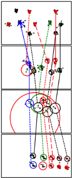
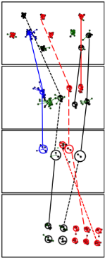
Figure 5 shows the MAP associations found by ICM and ICM-MCMC, with lines connecting cluster states over epochs. Annotations were also added (in the form of three different line styles) to facilitate comparison between the
(c) ICM (LL = -3329)
(d) MCMCDA (LL = -3365)
Figure 4: The clusters found for the simulated domain are shown in thick ellipses, centered at the location mean, color-coded by the most-likely object type inferred (across the entire trajectory, since it is a static attribute). The ellipses depict a level set of the posterior location distribution (uncertainty given by Gaussian covariance matrix). In contrast, the posterior clusters found by ICM and the most-likely sample from MCMC (of 105 ), shown in the bottom row, are qualitatively much different, and have significantly lower log-likelihood (LL) values.
ICM and ICM-MCMC results; see figure caption for details. ICM tends to suggest many more transitions than ICMMCMC, many of which are actually implausible.
7 Discussion
We have presented an extension of the clustering-based world modeling approach to semi-static environments, by applying the DDPMM. Multiple modifications on the generic DDPMM were necessary to adhere to assumptions in the world modeling problem. Additionally, because of the extra temporal dimension, inference is even more challenging. A fast approximate MAP inference algorithm, iterated conditional modes (ICM), was therefore explored. By itself, ICM did not perform well; a novel two-stage inference algorithm, with ICM followed by MCMCDA, fared much better, both in simulation and on real-world data.
(d) ICM-MCMC transitions not present in ICM
Figure 5: Approximate MAP cluster (object) trajectories found using ICM and ICM-MCMC on the robot vision data collection in Wong et al. [2015]. The concatenated sequence of scenes (epochs) is shown from top to bottom. The inferred clusters and tracks are shown in the middle two columns. Lines connecting cluster pairs between epochs are color-coded by the inferred object type (fixed across epochs), and are marked by one of three line styles used to compare results from the two algorithms. A solid line means the same pair was connected by both algorithms; a dashed line means a similar pair (in likelihood) was connected; a dotted line means the pair was not connected by the other algorithm. To make the differences clearer, the topdown reference views have been annotated with arrows, for pairs of objects that were only connected by one algorithm (dotted lines in the middle two). The left column shows pairs that were connected by ICM but not ICM-MCMC; the right column shows the opposite. Solid arrows depict transitions that are unlikely, whereas dashed arrows depict plausible transitions. ICM tends to suggest many more transitions than ICM-MCMC, many of which are actually implausible.
The downside of the ICM-MCMC inference procedure is that very few guarantees can be made, since ICM is itself approximate and only reaches a local optimum. Additionally, even though the second-stage MCMCDA provides samples, they are not true samples from the full posterior, since the 'data points' it is trying to connect are in fact clusters found by ICM. Nevertheless, the idea of splitting the inference into within-epoch and between-epoch stages is appealing. The between-epoch stage of joining clusters into tracks also has connections with split-merge methods (e.g., [Jain and Neal, 2004]). We are currently developing a two-stage sampling procedure that relies on the same intuition, but produces association samples from the true posterior distribution.
The inference algorithms presented in this paper, and other traditional tracking algorithms such as MHT, all consider each view in sequence, sampling/scoring correspondence vectors given the associations from all previous views, but not future ones. That is, they are all performing forward filtering/sampling, but no smoothing is done in the space of associations. In previous work, we showed cases where this may be problematic [Wong et al., 2015]. For sampling-based algorithms to be considered a true Gibbs sampler, it must condition on all information that is available to it, both past and future (if operating in batch mode, which is the case). We are currently developing a true Gibbs sampler for the DDPMM.
Framing data association as a clustering problem allows us to consider sophisticated machine learning algorithms, such as variational inference [Blei and Jordan, 2006], possibly leading to better and faster data association. We can also consider connections in the reverse direction, leading to new algorithms for dynamic clustering, such as using MCMCDA to perform inference in generic DDPMMs and other models.
8 Acknowledgments
We gratefully acknowledge support from NSF grants 1420927 and 1523767, from ONR grant N00014-14-1-0486, and from ARO grant W911NF1410433. Any opinions, findings, and conclusions or recommendations expressed in this material are those of the authors and do not necessarily reflect the views of our sponsors.
@inproceedings{ijcai2016p496,
  title     = {Object-Based World Modeling in Semi-Static Environments with Dependent Dirichlet Process Mixtures},
  author    = {Wong, Lawson L. S. and Kurutach, Thanard and Lozano-Perez, Tomas and Kaelbling, Leslie Pack},
  booktitle = {Proceedings of the Twenty-Fifth International Joint Conference on
               Artificial Intelligence, {IJCAI-16}},
  publisher = {AAAI Press / International Joint Conferences on Artificial Intelligence},
  editor    = {Subbarao Kambhampati},
  pages     = {3513--3520},
  year      = {2016},
  month     = {7},
  url       = {https://ijcai.org/proceedings/2016/496},
}
TY - CPAPER TI - Object-Based World Modeling in Semi-Static Environments with Dependent Dirichlet Process Mixtures AU - Wong, Lawson L. S. AU - Kurutach, Thanard AU - Lozano-Perez, Tomas AU - Kaelbling, Leslie Pack T2 - Proceedings of the Twenty-Fifth International Joint Conference on Artificial Intelligence, IJCAI-16 PB - AAAI Press / International Joint Conferences on Artificial Intelligence PY - 2016 SP - 3513 EP - 3520 UR - https://ijcai.org/proceedings/2016/496 ER -Copied
Machine-readable versions of this paper, for tools and AI agents:





